Welcome to pyBIA’s Documentation!
Documentation status (last updated May 19, 2026)
This documentation is actively being developed and may change.
pyBIA (Blob Identification Algorithm) is an open-source Python framework for automated detection and classification of spatially extended, diffuse emission at high redshift (i.e., blob-like sources), such as Lyman-alpha blobs (LABs). The software was developed to support the analysis in Godines and Prescott 2026. If you use pyBIA in a publication, we would appreciate citations to the paper as well as the software release DOI.
By integrating source detection, aperture photometry, morphological segmentation, and machine learning, pyBIA provides an end-to-end pipeline for reducing large source catalogs into a prioritized candidate list for follow-up study. While optimized for high-redshift astronomy, its modular architecture makes it a flexible software tool for workflows requiring image segmentation, anomaly detection, or classification.
Reproducibility
Stochastic processes (e.g., model initialization, data shuffling) are controlled by a global seed attribute, SEED_NO (1909 by default). You can override this during class initialization to enable reproducible runs (or set it to None for random runs). Note that while the classical machine-learning workflows are reproducible given a fixed seed, exact determinism for the deep-learning models will still vary unless deterministic TensorFlow settings are explicitly enabled.
Key Features
pyBIA is organized into four core modules that handle the image-based feature engineering as well as the subsequent training and optimization of the machine learning classifiers.
Extract sources using segmentation maps, compute morphological moments, and generate photometric/morphological catalogs.
Train robust classifiers (e.g., tree-based ensembles) with built-in BorutaSHAP feature selection and Optuna hyperparameter optimization.
Identify and remove imaging artifacts/outliers using Isolation Forests on extracted feature vectors (HOG, FFT, Wavelet).
Train pre-built CNN architectures (AlexNet, ResNet18, VGG16) on single or multi-band imaging (up to 5 channels), with automated augmentation and cross-validation.
Quick Start
Installation
pyBIA requires Python 3.12+. Install the latest stable release via pip:
pip install pyBIA
Alternatively, install the development version from GitHub:
git clone https://github.com/Professor-G/pyBIA.git
cd pyBIA
pip install .
Tutorial
This section summarizes the pyBIA codebase through simplified examples of the core modules. These examples show how imaging data are used to generate source catalogs and to train machine learning models for classification and anomaly detection.
The catalog module constructs photometric and segmentation-based morphological catalogs from single-band imaging. Catalog generation can be run in either targeted mode, where source centroids are provided, or detection mode, where sources are identified automatically when no coordinates are supplied. This example demonstrates initializing a Catalog with a 2D image (data) and uncertainty map (error), enabling background subtraction (``bkg``=None), and computing the photometric and morphological features.
import numpy as np
from pyBIA import catalog

# Generate test image with some background sky level
bkg_level = 100.0
data = np.random.normal(loc=bkg_level, scale=5.0, size=(1000, 1000))

# Inject two artificial sources (50, 400) and (612, 80)
data[400-5:400+5, 50-5:50+5] += 500
data[80-5:80+5, 612-5:612+5] += 500

# Generate a Poisson-like uncertainty map
error = np.sqrt(np.abs(data))

# Initialize the Catalog object
cat = catalog.Catalog(
    data=data,                  # 2D image (single band)
    error=error,                # 2D uncertainty map (same shape as data)
    bkg=None,                   # Background estimation; set to 0.0 for no subtraction
    exptime=30.0,               # Exposure time (s)
    x=[50, 612], y=[400, 80],   # Source centroid(s) (pix); set to None to detect source(s)
    invert=True,                # Flips the (x, y) coords when cropping sub-images, for data with (row, column) indexing
    zp=26.23, nsig=0.35,        # Photometric zero point and segmentation threshold
    obj_name=['Obj_A', 'Obj_B'] # Object name(s)
)

# Compute features and save catalog
cat.create(save_file=True, filename='my_catalog.csv')
This example demonstrates the ensemble_model interface for supervised classifier training. The Classifier class supports optional missing-data imputation and can be run with default hyperparameters or with automated tuning. When enabled, tuning applies BorutaSHAP feature selection followed by Optuna hyperparameter optimization using a cross-validated objective metric. Built-in class methods are available to visualize performance (plot_conf_matrix, plot_roc_curve), optimization results (plot_feature_opt, plot_hyper_opt, plot_hyper_param_importance), and feature space distributions (plot_tsne).
import numpy as np
from sklearn.datasets import make_classification
from pyBIA import ensemble_model

# Generate synthetic dataset
data_x, data_y = make_classification(
    n_samples=500,
    n_features=62,
    n_informative=5,
    n_redundant=2,
    random_state=42
)

# Initialize the Classifier with features (data_x) and labels (data_y)
model = ensemble_model.Classifier(
    data_x=data_x,              # Feature matrix of shape (n_samples, n_features)
    data_y=data_y,              # 1D array of labels aligned to data_x
    clf='xgb',                  # The classification model to train
    impute=True,                # Whether to impute missing feature values
    optimize=True,              # Enables automated feature selection & hyperparameter tuning
    n_iter=50,                  # Number of Optuna trials; set to 0 to skip
    scoring_metric='f1',        # Optuna objective (e.g., 'f1', 'precision', 'roc_auc')
    opt_cv=10,                  # Number of CV folds used during optimization
    boruta_trials=100,          # Number of BorutaSHAP trials; set to 0 to skip
    boruta_model='rf'           # Base estimator for BorutaSHAP feature ranking
)

# Run the optimization/training pipeline and save
model.create()
model.save(dirname='optimized_xgboost')
The following example demonstrates use of the outlier_detection module for unsupervised anomaly detection with an Isolation Forest. The Classifier optionally normalizes input cutouts and imputes missing feature values, computes a user-selected set of image descriptors, and fits an Isolation Forest on the resulting feature matrix. The trained model can then be applied to candidate cutouts to return outlier labels and anomaly scores.
import numpy as np
from pyBIA import outlier_detection

# Generate mock image cutouts
data = np.random.normal(loc=0.5, scale=0.1, size=(100, 32, 32, 1))

# Train an Isolation Forest on the single class
model = outlier_detection.Classifier(
    data=data,                  # Single-class image cutouts, shape: (N, H, W, C)
    img_num_channels=1,         # Set to C for multi-channel inputs
    feat_set='hog',             # Feature set to use
    clf='iforest',              # The unsupervised engine to train
    normalize=True,             # Whether to min-max normalize prior to feature extraction
    min_pixel =0, max_pixel=10, # Min and max pixel values for normalization
    impute=True                 # Whether to impute missing feature values
)

# Run the training pipeline and save
model.create()
model.save(dirname='outlier_model')
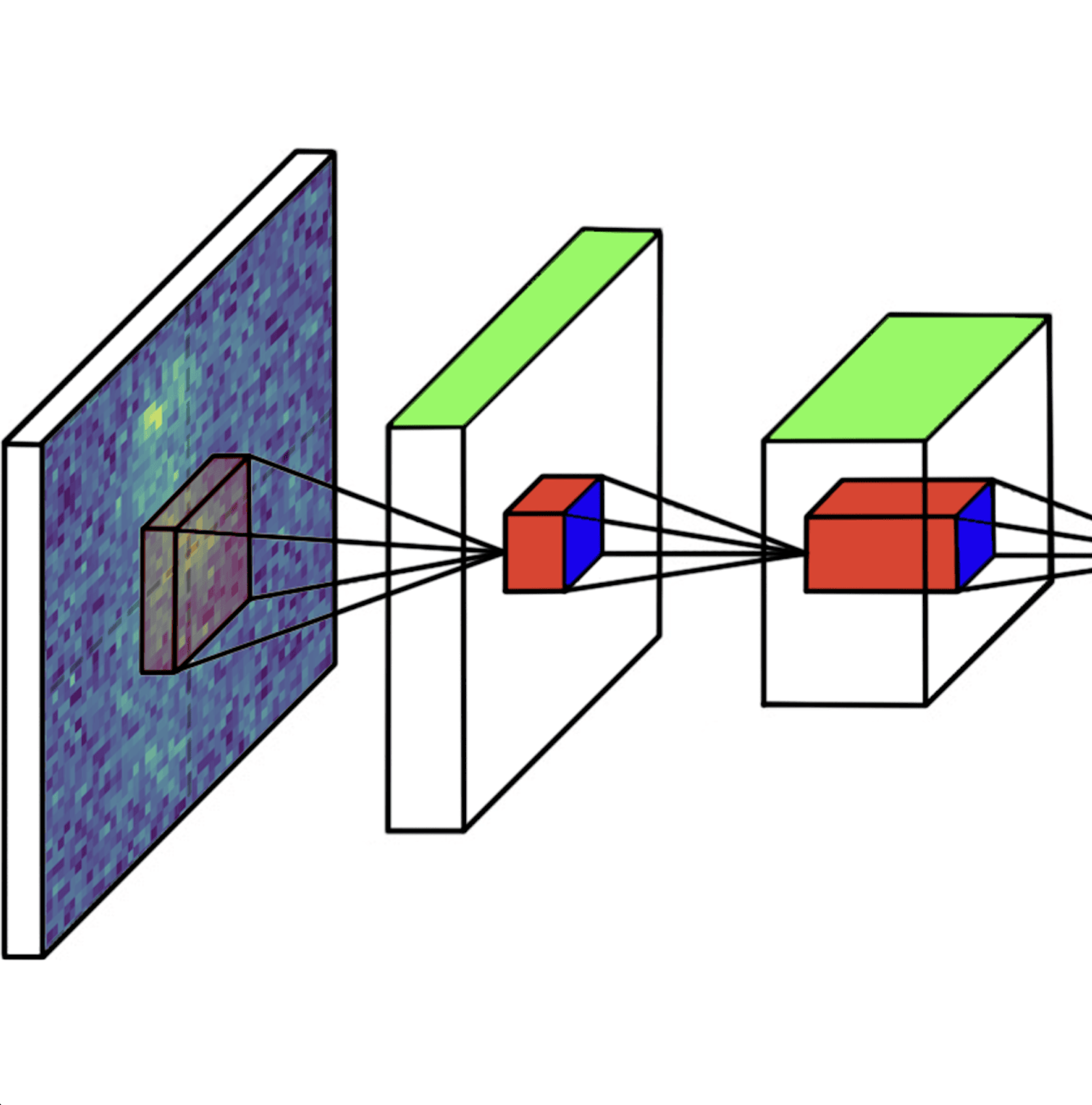
This final example provides an overview of the cnn_model module for image-based binary classification using convolutional neural networks. The Classifier accepts positive and negative-class cutouts (single or multi-channel), and optionally applies per-channel min-max normalization and data augmentation. When validation data is provided, the model can be trained using cross-validation, yielding an ensemble of fold-specific networks. Per-fold performance can be visualized via the plot_performance class method.
import numpy as np
from pyBIA import cnn_model

# Generate some image cutouts
pos_class = np.clip(np.random.normal(loc=60, scale=10, size=(200, 64, 64, 1)), 0, 100)
neg_class = np.clip(np.random.normal(loc=40, scale=10, size=(200, 64, 64, 1)), 0, 100)
val_pos = np.clip(np.random.normal(loc=60, scale=10, size=(50, 64, 64, 1)), 0, 100)
val_neg = np.clip(np.random.normal(loc=40, scale=10, size=(50, 64, 64, 1)), 0, 100)

# Initialize the Classifier with validation data
model = cnn_model.Classifier(
    positive_class=pos_class,   # Positive class cutouts, shape: (N, H, W) or (N, H, W, C)
    negative_class=neg_class,   # Negative class cutouts
    val_positive=val_pos,       # Positive validation cutouts
    val_negative=val_neg,       # Negative validation cutouts
    img_num_channels=1,         # Set to C for multi-channel inputs
    clf='alexnet',              # Model to train
    normalize=True,             # Whether to apply per-channel min-max scaling
    min_pixel=0,                # Minimum pixel for normalization
    max_pixel=100,              # Maximum pixel for normalization (or list for multi-channel)
    augment_data=True,          # Whether to augment the training data
    batch_positive=10,          # Number of augmentations per positive instance
    batch_negative=0,           # Number of augmentations per negative instance
    epochs=3, batch_size=16,    # Training epochs and mini-batch size
    optimizer='sgd', lr=1e-4,   # Optimizer and learning rate
    patience=3,                 # Patience parameter for early-stopping
    opt_cv=5,                   # Cross-validation folds; set to None for a single model
    activation_conv='relu',     # Activation function for the Conv2D layers
    activation_dense='relu'     # Activation function for the fully connected (dense) layers
)

# Run the data augmentation/training pipeline and save
model.create()
model.save(dirname='alexnet_model')
Citation
If you use pyBIA in your research, please cite the paper and the Zenodo DOI:
User Guide
The pages below provide tutorials, API references, and high-level technical details on the program’s core functionality, as well as a dedicated section describing how Godines and Prescott 2026 was produced, including figure-by-figure generation details.
Core Modules
Case Studies
API Reference