Morphological Catalog

The catalog module is the core of pyBIA’s morphological feature extraction and catalog-generation pipeline. It performs source detection, aperture photometry, and segmentation-based morphology measurements designed for training machine-learning models. This is all handled by the Catalog class.

This module combines image segmentation (via Astropy’s photutils) with moment-based descriptors (included in the image_moments module) to convert image data into a feature matrix containing:

Photometry: aperture fluxes and flux errors (and magnitudes if a zeropoint is provided).
Moments: raw, central, geometrically centered, Hu-invariant, and Legendre moments computed on the segmented source.
Segmentation properties: shape and intensity statistics (e.g., ellipticity, eccentricity, Gini, bounding box and other metadata).

Quick Start

Automatic detection (no input positions)

If you provide a 2D image containing various sources and do not specify positions, pyBIA will run segmentation on the full frame and build a catalog for all detected sources:

from pyBIA import catalog

# Instantiate the Catalog class (data is the image array)
cat = catalog.Catalog(data)

# Run source detection and compute photometric and morphological features
cat.create(save_file=True)

# The catalog is stored in the ``cat.cat`` attribute
print(cat.cat)

Targeted extraction (user-supplied positions)

If you want to analyze a specific source (or a set of sources) at known pixel positions, pass the x and y arguments, which represent the source coordinate(s), in relative pixels of the input image:

from pyBIA import catalog

# Example: 100x100 stamp with a source at the center
cat = catalog.Catalog(data, x=50, y=50)
cat.create(save_file=True)

print(cat.cat)

Computed Features

When morph_params=True (default), pyBIA returns a morphology vector containing various source properties including segmentation-based image moments.

Moments are computed on the segmented source pixels (all non-source pixels are zeroed prior to measurement). The moments table contains 47 features:

Raw moments up to 3rd order:

M00, M10, M01, M20, M11, M02, M30, M21, M12, M03

Central moments up to 3rd order:

mu00, mu10, mu01, mu20, mu11, mu02, mu30, mu21, mu12, mu03

Geometrically centered polynomial moments up to 3rd order:
```
G00, G10, G01, G20, G11, G02, G30, G21, G12, G03
```
Hu invariants:
```
Hu1, Hu2, Hu3, Hu4, Hu5, Hu6, Hu7
```
Legendre moments (orthonormal) up to total order 3 (n+m ≤ 3):
```
L00, L10, L01, L20, L11, L02, L30, L21, L12, L03
```

Shape/geometry:

eccentricity, ellipticity, elongation, orientation, perimeter, equivalent_radius, fwhm

Intensity/statistics:

gini, max_value, min_value, plus index metadata for extrema

Covariance/ellipse terms:

covar_sigx2, covar_sigy2, covar_sigxy, cxx, cxy, cyy, covariance_eigval1, covariance_eigval2

Bounds:

bbox_xmin, bbox_xmax, bbox_ymin, bbox_ymax

Scalar flag:

isscalar (stored as 1 for True, 0 for False)

In total, the default morphology vector contains 77 features per source (47 moment features + 30 segmentation properties), plus optional photometry and metadata columns (e.g., flux, flux_err, mag, mag_err, median_bkg, xpix, ypix, obj_name, field_name, flag), depending on which inputs are provided (e.g., zp, error, bkg, and position mode).

Methodology

Catalog generation follows one of two workflows depending on whether positions are provided:

Auto-detect mode (`x`/`y` not provided)

Background subtraction (optional): if bkg=None, a robust global/tiled sigma-clipped background is subtracted from the full frame prior to segmentation.
Segmentation: the background-subtracted image is convolved with a Gaussian kernel (FWHM = 9 pixels; window size set by kernel_size), then thresholded at nsig using photutils.detect_sources (with an option to deblend the detected sources).
Photometry: circular-aperture photometry is measured at the detected centroids using radius aperture (pixels).
Morphology: for each detected centroid, a local square cutout of length size is extracted and morphology features are computed on the segmented pixels.

Targeted mode (`x`/`y` provided)

When positions are input, pyBIA treats each coordinate pair as an independent source/measurement:

Photometry: circular-aperture flux is measured at (x, y) using radius aperture (pixels). If bkg=None, a sigma-clipped annulus median (radii annulus_in and annulus_out in pixels) is used for local background subtraction and stored as median_bkg.
Cutout extraction: a square cutout of length size is cropped around the target coordinate (automatically reduced if the image is smaller than size).
Segmentation (cutout): the cutout is convolved with the Gaussian kernel and segmented using the same nsig/kernel_size/npixels/connectivity settings (with optional deblend). If exptime is provided, the cutout is divided by exptime for segmentation and morphology only (photometry is measured on the original data).
Central validation: the detection is accepted only if a segmented region is present near the cutout center. If threshold==0, the central pixel must lie in the segmentation; otherwise, at least one segmented pixel must fall within a central circular mask of radius threshold. The segmented object whose centroid is closest to the cutout center is retained.
Morphology: moment features and segmentation properties are computed on the retained segmented pixels. If validation fails, morphology columns are set to -999 while photometry is still reported.

Key Parameters

The Catalog class includes the following parameters:

Parameter	Default	Description
`x`, `y`	`None`	Source center pixel coordinates. If `None`, pyBIA runs automatic detection on the full frame.
`bkg`	`None`	Background handling. Use `0` if the image is already background-subtracted; use `None` to estimate local background (targeted mode) or subtract a global background (auto-detect mode).
`error`	`None`	Optional per-pixel error map (same shape as `data`). Enables `flux_err` and `mag_err`.
`zp`	`None`	Zeropoint for magnitude calculation. If provided, `mag` and `mag_err` are computed from aperture fluxes.
`exptime`	`None`	Exposure time (seconds). If provided, cutouts are divided by `exptime` for segmentation/morphology (photometry is measured on the original data).
`morph_params`	`True`	If `True`, compute morphology features (moments + segmentation properties). If `False`, only photometry/metadata columns are produced.
`nsig`	`0.3`	Segmentation detection threshold (in sigma above background).
`threshold`	`10`	Central validation radius (pixels). Use `0` to require exact central-pixel membership in a segment.
`deblend`	`False`	If `True`, attempt to split overlapping sources during segmentation.
`size`	`100`	Side length (pixels) of the square cutout used to segment each source when computing morphology.
`aperture`	`15`	Circular-aperture radius (pixels) for photometry.
`annulus_in`	`20`	Inner radius (pixels) of the background annulus (targeted mode; `bkg=None`).
`annulus_out`	`35`	Outer radius (pixels) of the background annulus.
`kernel_size`	`21`	Gaussian convolution window size (pixels) used prior to segmentation.
`npixels`	`9`	Minimum number of connected pixels required to define a detection.
`connectivity`	`8`	Pixel connectivity (4 = edge-connected, 8 = edge+corner-connected).
`invert`	`False`	If `True`, swap (x, y) ordering when cropping cutouts (useful for row/column-style indexing).

Note

Non-detections (morphology): if the segmentation does not contain a valid central object, pyBIA flags the source as a non-detection and sets all morphology columns to -999. Aperture photometry is still recorded.

Example

In this example, we generate a source catalog for a dataset of 20,000 simulated extragalactic sources (10k strong gravitational lenses, 10k non-lensed galaxies). These sources are simulated in the five bands LSST will observe (g, r, i, z, y).

Data Access You can download the sample binary files here:

Processing Script We will process each band individually, constructing separate catalogs for lenses and non-lenses, and then merging them.

import numpy as np
import pandas as pd
from pyBIA import catalog

# Load the images, binary files (41x41 pixels) containing five filters: g,r,i,z,y
lenses = np.load('lenses_10k.npy')
nonlenses = np.load('nonlenses_10k.npy')

# pyBIA catalog parameteres #

error = None # The corresponding error map, for computing photometric errors
xpix = ypix = lenses.shape[-1] // 2 # Relative position (in pixels) of the source centroid, here they are centered about the image cutouts
bkg = None # None if background subtraction required, else set to 0 if data already bg-subtracted
aperture = 10 # Aperture radius (in pixels) for the photometry
annulus_in = 15 # Inner radius (in pixels) of background annulus for local sky estimation
annulus_out = 50 # Outer radius (in pixels) of background annulus.
nsig = 0.3 # The image segmentation detection threshold
threshold = 1 # Will plot the closest object within a circular mask of radius 1 (pixels) within the center
exptime = 1 # Exposure time to normalize the flux
zp = 27 # The instrumental zeropoint, for computing the apparent magnitudes
deblend = False # Whether to deblend detected source(s)
kernel_size = 21 # Gaussian filter kernel size used to convolve the data prior to segmentation
npixels = 9 # Required number of pixels above the sigma threshold required to detect a source
connectivity = 8 # Scheme to determine how pixels are grouped into a detected source, either 4 (touch along edges) or 8 (edges and corners)

# Will process one band at a time, and save each individually
for i, band in enumerate(['g','r','i','z','y']):

        # To save all of the individual catalogs
        master_catalog = []

        # Loop through each individual lens source
        for j in range(len(lenses)):
                obj_name = j # The object name in the catalog will just be the order as it appears in the data
                flag = 1 # The positive class label

                # Instantiate the Catalog class
                cat = catalog.Catalog(
                        data=lenses[j][i], # First axis selects the individual source, second axis the band
                        error=error,
                        x=xpix,
                        y=ypix,
                        bkg=bkg,
                        aperture=aperture,
                        annulus_in=annulus_in,
                        annulus_out=annulus_out,
                        nsig=nsig,
                        threshold=threshold,
                        exptime=exptime,
                        zp=zp,
                        deblend=deblend,
                        kernel_size=kernel_size,
                        npixels=npixels,
                        connectivity=connectivity,
                        obj_name=obj_name,
                        flag=flag
                        )

                # Create the catalog, will be stored as the `cat` class attribute.
                cat.create(save_file=False)

                # Append the created `cat` attribute to the master list
                master_catalog.append(cat.cat)

        ##
        ## Now repeat for the non-lenses ##
        ##

        # Loop through each individual non-lens source
        for j in range(len(nonlenses)):
                obj_name = len(lenses) + j # The object name in the catalog will just be the order as it appears in the data + how many lenses there are already
                flag = 0 # The negative class label

                # Instantiate the Catalog class
                cat = catalog.Catalog(
                        data=nonlenses[j][i], # First axis selects the individual source, second axis the band
                        error=error,
                        x=xpix,
                        y=ypix,
                        bkg=bkg,
                        aperture=aperture,
                        annulus_in=annulus_in,
                        annulus_out=annulus_out,
                        nsig=nsig,
                        threshold=threshold,
                        exptime=exptime,
                        zp=zp,
                        deblend=deblend,
                        kernel_size=kernel_size,
                        npixels=npixels,
                        connectivity=connectivity,
                        obj_name=obj_name,
                        flag=flag
                        )

                # Create the catalog, will be stored as the `cat` class attribute.
                cat.create(save_file=False)

                # Append the created `cat` attribute to the master list
                master_catalog.append(cat.cat)


        # Now Merge all individual catalogs into one master dataframe and save
        df = pd.concat(master_catalog, ignore_index=True)
        df.to_csv(f'segm_catalog_{band}_band.csv', index=False)

The five catalogs generated above are available for download here:

These catalogs will be merged and used to train a binary classifier using the ensemble_model module. This example is provided in the Supervised Learning Algorithms page.

NOTE: The catalog module also provides a standalone function to plot individual sources and the corresponding image segmentation patches given some set of parameter(s). The plot_objects_segmentation function allows users to inspect the segmentation masks overlaid on the source. As the source morphological features are dependent on the resulting segmentation, it is important to ensure the generated patches are truly representative of the source morphology. This function allows users to input up to four segmentation detection thresholds (sigma_values), so as to visualize how different values affect the resulting source extent.

In the example below, we inspect a lens where only the i-band yields a positive detection at the strictest threshold (\(\sigma=5.0\)). The other four filters at this detection level would be non-detections and the corresponding morphological features would thus be cataloged with -999 values.

import numpy as np
from pyBIA import catalog

# Load the lenses
lens = np.load('lenses_10k.npy')

# Plotting parameters
median_bkg = None # Whether to subtract the background (set to None if background subtraction required)
pix_conversion = 5.8 # Survey pixel-per-arcsecond (for setting the axes)
crop_size = None # Will crop the image to be of this size, otherwise set to None
xpix = ypix = lens.shape[2] // 2 # Cropped image will be centered about these coords, if not cropping set to None
r_in = 15 # Inner radius (in pixels) of background annulus for local sky estimation
r_out = 50 # Outer radius (in pixels) of background annulus.

# Figure parameters
fig_title = r'Example Lens' # Figure suptitle
sup_titles = [r'$g$', r'$r$', r'$i$', r'$z$', r'$y$'] # Title(s) above each individual panel
cmap = 'viridis' # Colormap to use when displaying input image, the segmentation patches always use binary

# Segm detection parameters
sigma_vals = [0.3, 1.0, 3.0, 5.0] # The detection threshold(s) to apply
deblend = False # Whether to deblend detected sources
kernel_size = 21 # Gaussian filter kernel size used to convolve the data prior to segmentation
npixels = 9 # Required number of pixels above the sigma threshold required to detect a source
connectivity = 8 # Scheme to determine how pixels are grouped into a detected source, either 4 (touch along edges) or 8 (edges and corners)
threshold = 0 # Will plot the object present within the image center
savefig = True # Whether to save the figure, it False it will show instead
savepath = 'segm_example_lens.png' # Path (and/or filename) to save in/as

i = 4 # Will plot the fifth source in the array

# This function takes in up to 5 images, and plots the detection thresholds (up to 4 thresholds allowed)
catalog.plot_objects_segmentation(
   lens[i][0],
   lens[i][1],
   lens[i][2],
   lens[i][3],
   lens[i][4],
   pix_conversion=pix_conversion,
   sigma_values=sigma_vals,
   deblend=deblend,
   kernel_size=kernel_size,
   npixels=npixels,
   connectivity=connectivity,
   threshold=threshold,
   titles=sup_titles,
   suptitle=fig_title,
   cmap=cmap,
   xpix=xpix,
   ypix=ypix,
   size=crop_size,
   median_bkg=median_bkg,
   savefig=savefig,
   r_in=15,
   r_out=50,
   savepath=savepath
   )

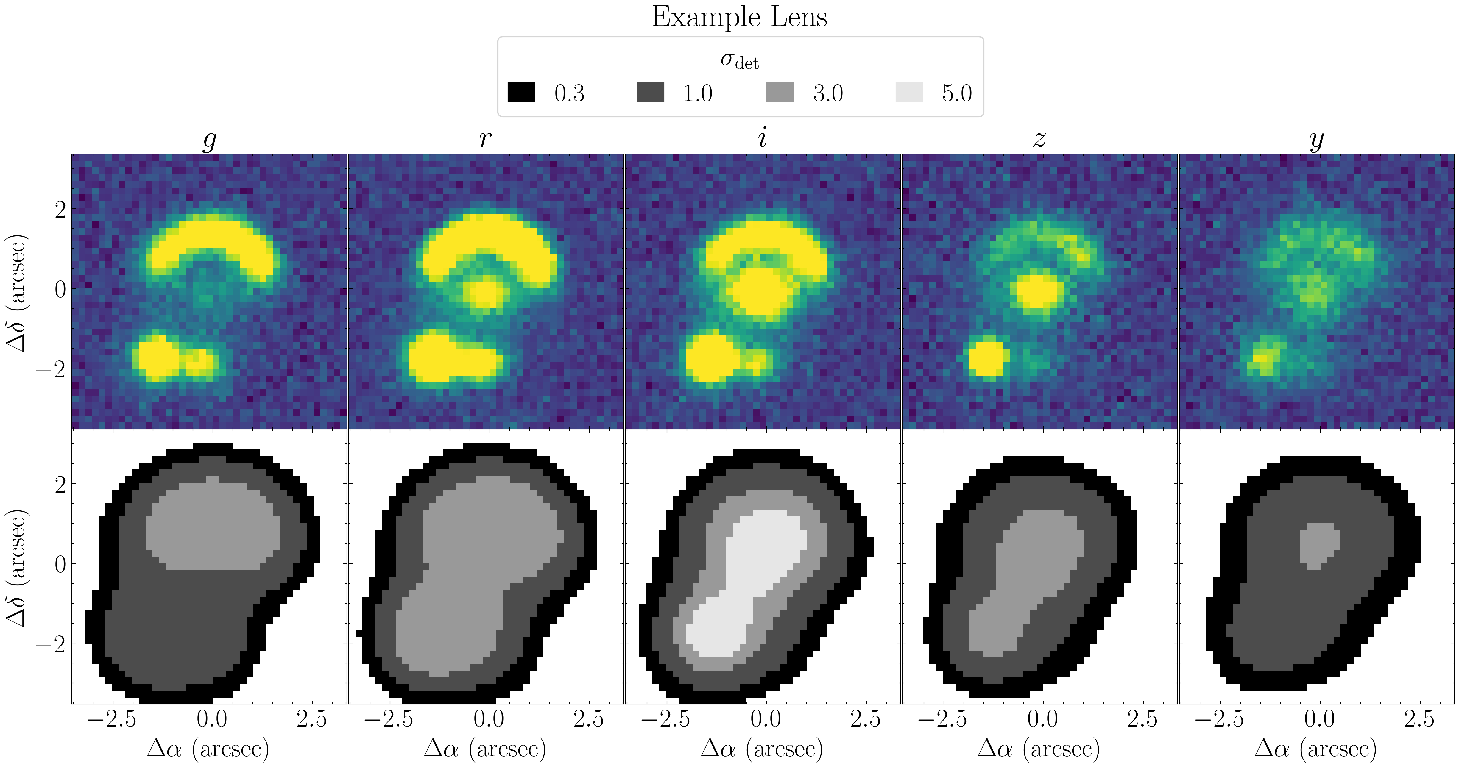
Segmentation Example — Visualization of segmentation maps across 5 bands. The binary masks illustrate the detected morphology at increasing sigma thresholds, computed from the `sigma_values`.