Godines & Prescott (2026)
This page provides all of the code necessary to reproduce the analysis presented in Godines and Prescott 2026. The core modules of pyBIA handle the heavy computational work, while the scripts in this documentation serve as the front end. If anything is unclear, please feel free to contact me by email: danielgodinez123@gmail.com.
The associated data products are supplied incrementally within the scripts to enable step-by-step analysis and the replication of individual stages in a transparent, technical manner. For convenience, we also provide direct access to the complete and priority catalogs below.
Our complete catalog of the Boötes field (~2.4 million sources), including probability prediction scores from the three machine learning models and the morphological features computed from the Bw imaging, is available for download here.
A sub-catalog containing the 110 priority candidates is available here, along with the corresponding Bw and R-band imaging data, which can be downloaded as a binary file here.
NOTE: All figures are formatted using the scienceplots Python package, available via pip.
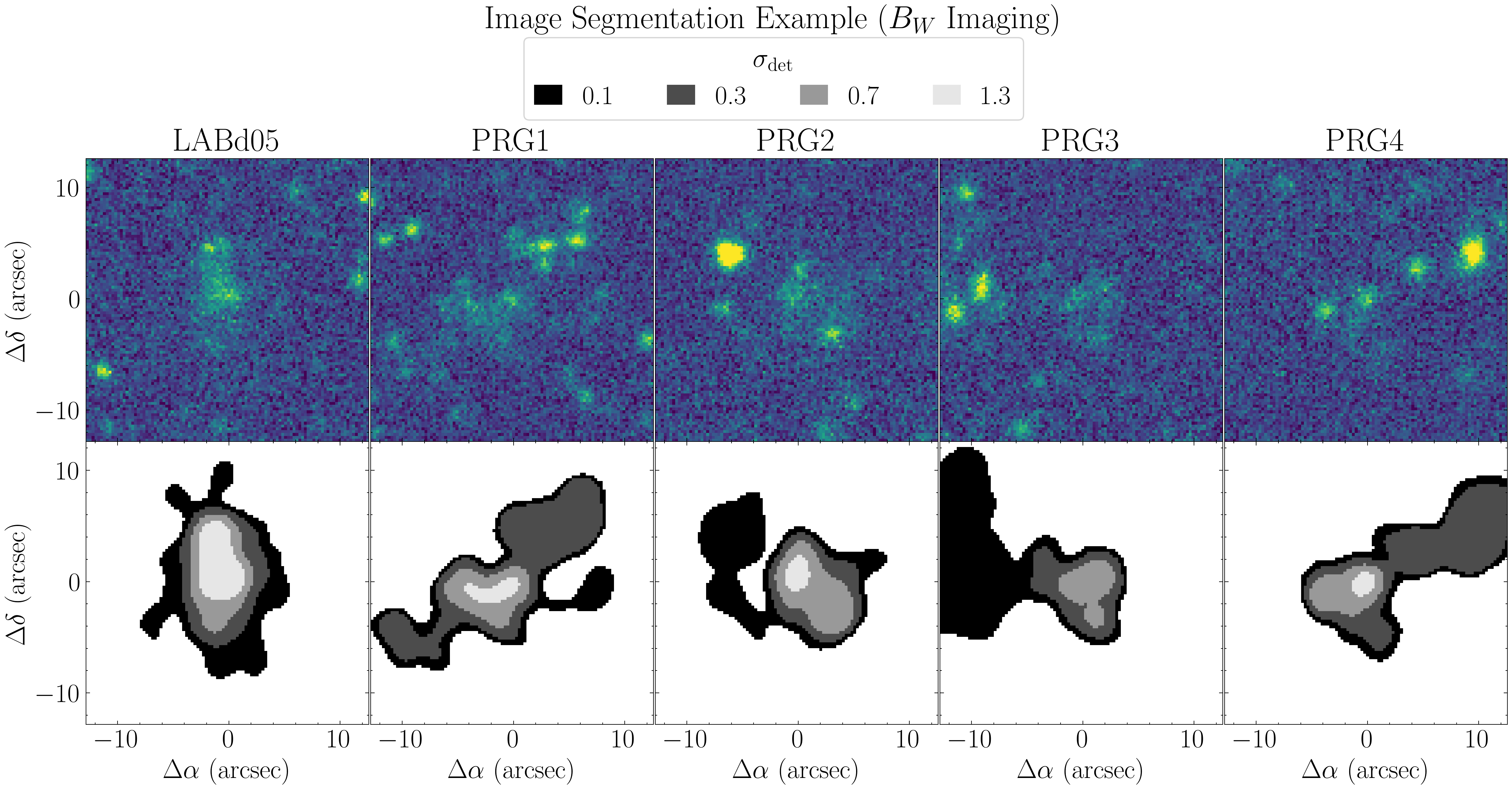
Image Segmentation
The multi-band data (Bw and R) for the five broadband-selected Lyman-α blobs (LABs) from Prescott et al 2012 can be downloaded here.
The corresponding NDWFS Boötes Survey catalog names for these five objects can be downloaded here.
To visualize how varying the sigma-detection threshold affects the resulting image segmentation, use the plot_objects_segmentation function available in the catalog module.
import numpy as np
from pyBIA import catalog

# Load the five broadband-selected LABs from Prescott+12
five_confirmed = np.load('confirmed_LAB.npy')

# These are the Bw images, second axis contains the R-band data
five_confirmed_bw = five_confirmed[:,:,:,0]

# The corresponding cataloged names
names = np.loadtxt('confirmed_LAB_names.txt', dtype=str)

# Index the images of each LAB according to its cataloged name
PRG1 = five_confirmed_bw[(names == 'NDWFS_J143512.2+351108')][0]
PRG2 = five_confirmed_bw[(names == 'NDWFS_J142623.0+351422')][0]
PRG3 = five_confirmed_bw[(names == 'NDWFS_J143412.7+332939')][0]
PRG4 = five_confirmed_bw[(names == 'NDWFS_J142653.1+343856')][0]
LABd05 = five_confirmed_bw[(names == 'NDWFS_J143410.9+331730')][0]

# Plotting parameters
median_bkg = 0 # Whether to subtract the background (set to None if background subtraction required)
pix_conversion = 3.8961 # NDWFS survey pixel-per-arcsecond (for setting the axes)
crop_size = 100 # Will crop the image to be of this size, otherwise set to None
xpix = ypix = five_confirmed.shape[1] // 2 # Cropped image will be centered about these coords, if not cropping set to None

# Figure parameters
fig_title = r'Image Segmentation Example ($B_W$ Imaging)' # Figure suptitle
sup_titles = ['LABd05', 'PRG1','PRG2','PRG3','PRG4'] # Title(s) above each individual panel
cmap = 'viridis' # Colormap to use when displaying input image, the segmentation patches always use binary

# Segm detection parameters
sigma_vals = [0.1, 0.3, 0.7, 1.3] # The detection threshold(s) to apply
deblend = False # Whether to deblend detected sources
kernel_size = 21 # Gaussian filter kernel size used to convolve the data prior to segmentation
npixels = 9 # Required number of pixels above the sigma threshold required to detect a source
connectivity = 8 # Scheme to determine how pixels are grouped into a detected source, either 4 (touch along edges) or 8 (edges and corners)
threshold = 10 # Will plot the closest object within a circular mask of radius 10 (pixels) within the center
savefig = True # Whether to save the figure, it False it will show instead
savepath = 'segm_example_LAB.png' # Path (and/or filename) to save in/as

# This function takes in up to 5 images, and plots the detection thresholds (up to 4 thresholds allowed)
catalog.plot_objects_segmentation(
    np.flip(LABd05, axis=0),
    np.flip(PRG1, axis=0),
    np.flip(PRG2, axis=0),
    np.flip(PRG3, axis=0),
    np.flip(PRG4, axis=0),
    pix_conversion=pix_conversion,
    sigma_values=sigma_vals,
    deblend=deblend,
    kernel_size=kernel_size,
    npixels=npixels,
    connectivity=connectivity,
    threshold=threshold,
    titles=sup_titles,
    suptitle=fig_title,
    cmap=cmap,
    xpix=xpix,
    ypix=ypix,
    size=crop_size,
    median_bkg=median_bkg,
    savefig=savefig,
    savepath='segm_example_LAB.png'
    )
Training Morphological Catalog
To access the archival data products used in this study, please visit the NoirLab website. We used the Boötes field catalog and imaging datasets, which cover 27 total subfields. The imaging data required to reproduce our full analysis has also been compiled for convenience and is available for download here.
The training-set objects used in our study can be downloaded here. This file contains catalog information for the 866 LAB candidates compiled by Prescott et al 2012, along with 3,200 randomly selected OTHER sources from the same dataset.
The code below demonstrates how we performed our detection-threshold analysis. Using the catalog information provided in the training set, we extracted morphological features via image segmentation at thresholds ranging from 0.1 to 1.5 standard deviations above the background RMS.
import numpy as np
import pandas as pd
from astropy.io import fits
from sklearn.model_selection import cross_validate
from pyBIA import catalog

### Create the Data Files to Generate Figure 2 ###

# This is where the subfield fits files are stored including the error maps
data_path = 'NDWFS/fits_images/Bw_FITS/'
data_error_path = 'NDWFS_Bootes/Error_Maps/Bw/'

#866 LAB candidates from Prescott et al. (2012) plus 3200 randomly selected OTHER objects
training_set = pd.read_csv('training_set.csv')

# The training features will be computed using the following varying sigma thresholds
sigs = np.around(np.arange(0.1, 1.51, 0.01), decimals=2)

# Where the training set files will be saved
nsig_path = 'nsigs/'

deblend = False # Whether to deblend detected sources
kernel_size = 21 # Gaussian filter kernel size used to convolve the data prior to segmentation
npixels = 9 # Required number of pixels above the sigma threshold required to detect a source
connectivity = 8 # Scheme to determine how pixels are grouped into a detected source, either 4 (touch along edges) or 8 (edges and corners)
threshold = 10 # Will plot the closest object within a circular mask of radius 10 (pixels) within the center
invert = True # Flips the (x, y) input order when cropping sub-images

for sig in sigs:
        print(sig)
        frame = [] #To store all 27 subfields
        for fieldname in np.unique(np.array(training_set['field_name'])):

                # Load the field data
                data_hdu, error_map = fits.open(data_path+fieldname+'_Bw_03_fix.fits'), fits.getdata(data_error_path+fieldname+'_Bw_03_rms.fits.fz')

                # Extract the data and corresponding ZP
                data_map, zeropoint, exptime = data_hdu[0].data, data_hdu[0].header['MAGZERO'], data_hdu[0].header['EXPTIME']

                # Select only the samples from this subfield
                subfield_index = np.where(training_set['field_name']==fieldname)[0]
                xpix, ypix = training_set[['xpix', 'ypix']].iloc[subfield_index].values.T
                objname, field, flag = training_set[['obj_name', 'field_name', 'flag']].iloc[subfield_index].values.T

                # Create the catalog object
                cat = catalog.Catalog(
                        data_map,
                        error=error_map,
                        x=xpix,
                        y=ypix,
                        zp=zeropoint,
                        exptime=exptime,
                        nsig=sig,
                        flag=flag,
                        obj_name=objname,
                        field_name=field,
                        deblend=deblend,
                        kernel_size=kernel_size,
                        npixels=npixels,
                        connectivity=connectivity,
                        threshold=threshold,
                        invert=invert
                        )

                # Generate the catalog and append the ``cat`` attribute to the frame list
                cat.create(save_file=False)
                frame.append(cat.cat)

        # Combine all 27 sub-catalogs into one master frame and save
        frame = pd.concat(frame, axis=0, join='inner')
        frame.to_csv(f'{nsig_path}_Bw_training_set_nsig_{sig}.csv', index=False)
All 141 nsig files have been compiled for convenience and are available for download here.
Baseline Classification Models
The files generated in the previous steps will be used to build our baseline classifiers using the ensemble_model module. These datasets provide the training and validation inputs necessary to evaluate model performance and establish a benchmark for subsequent analyses.
import numpy as np
import pandas as pd
from sklearn.model_selection import cross_validate, StratifiedKFold
from pyBIA import data_processing, ensemble_model, optimization

SEED_NO = 1909  # Fixed seed to initialize all random processes, including NumPy's RNG

# The training features were computed using the following varying sigma thresholds
sigs = np.around(np.arange(0.1, 1.51, 0.01), decimals=2)

# Where the training set files were saved
nsig_path = 'nsigs/'

#These are the features to use, note that the catalog includes more than this!
#Removing mu00 and G00 since these will be the same as M00
#Also removing mu10 and mu01 since these should be zero but in practice they are not but are very small
#due to floating-point precision errors and minor asymmetries in the image; thus contribute little meaningful variance for classification.
columns = [
    'mag', 'mag_err',
    'M00', 'M10', 'M01', 'M20', 'M11', 'M02', 'M30', 'M21', 'M12', 'M03',
    'mu20', 'mu11', 'mu02', 'mu30', 'mu21', 'mu12', 'mu03',
    'G10', 'G01', 'G20', 'G11', 'G02', 'G30', 'G21', 'G12', 'G03',
    'Hu1', 'Hu2', 'Hu3', 'Hu4', 'Hu5', 'Hu6', 'Hu7',
    'L00', 'L10', 'L01', 'L20', 'L11', 'L02', 'L30', 'L21', 'L12', 'L03',
    'area', 'covar_sigx2', 'covar_sigy2', 'covar_sigxy', 'covariance_eigval1', 'covariance_eigval2',
    'cxx', 'cxy', 'cyy', 'eccentricity', 'ellipticity', 'elongation',
    'equivalent_radius', 'fwhm', 'gini', 'orientation', 'perimeter',
    'semimajor_sigma', 'semiminor_sigma', 'max_value', 'min_value'
]

# To store the baseline performance as a function of sigma threshold for all classifiers, note that nn corresponds to MLP in the paper
classifiers = ['tree', 'rf', 'xgb', 'logreg', 'svc', 'nn']
all_metrics = {clf: {'nsig': [], 'accuracy': [], 'f1': [], 'precision': [], 'recall': [], 'roc_auc': []} for clf in classifiers}

blob_nondetect, other_nondetect = [], [] # To store the number of non-detections (Right Panel of Figure 2)
impute = False # Will not impute NaN values, as they should not be present after masking non-detections
num_cv_folds = 10 # Will assess the model's accuracy using 10-fold CV

###  Read the Data Files ###
for sig in sigs:
        print(sig)
        # Load the corresponding nsig file
        df = pd.read_csv(f'{nsig_path}_Bw_training_set_nsig_{sig}')

        # Log-transform the Hu moments
        hu_cols = ['Hu1', 'Hu2', 'Hu3', 'Hu4', 'Hu5', 'Hu6', 'Hu7']
        df[hu_cols] = df[hu_cols].apply(data_processing.signed_log_transform)

        # Omit any non-detections (nan mags (~10%) and nan Hu moments (~0.02%))
        mask = np.where((df['area'] != -999) & np.isfinite(df['mag']) & np.all(np.isfinite(df[[f'Hu{i}' for i in range(1, 8)]]), axis=1))[0]

        # Balance both classes to be of same size
        blob_index = np.where(df['flag'].iloc[mask] == 1)[0]
        other_index = np.where(df['flag'].iloc[mask] == 0)[0]
        df_filtered = df.iloc[mask[np.concatenate((blob_index, other_index[:len(blob_index)]))]]

        # Feature matrix and labels array
        data_x, data_y = np.array(df_filtered[columns]), np.array(df_filtered['flag'])

        # Instantiate the Classifier class
        model = ensemble_model.Classifier(data_x, data_y, impute=impute)

        for clf_name in all_metrics.keys():
                # The last three in the list, these classifiers require the training data to be standardized
                if clf_name in ['logreg', 'svc', 'nn']:
                        model.data_x = optimization.standardize_data(data_x, method='standard', return_scaler=False)
                else:
                        model.data_x = data_x

                model.clf = clf_name
                model.create(overwrite_training=False)

                # 10 fold CV, save multiple metrics
                cv_splitter = StratifiedKFold(n_splits=num_cv_folds, shuffle=True, random_state=SEED_NO)
                cross_val = cross_validate(model.model, model.data_x, model.data_y, cv=cv_splitter, scoring=['accuracy', 'f1', 'precision', 'recall', 'roc_auc'])

                # Append nsig and scores
                all_metrics[clf_name]['nsig'].append(sig)
                for metric in ['accuracy', 'f1', 'precision', 'recall', 'roc_auc']:
                        all_metrics[clf_name][metric].append(np.mean(cross_val[f'test_{metric}']))

        # This checks how many normalized non-detections occurred at this threshold
        blob_index, other_index = np.where(df['flag'] == 1)[0], np.where(df['flag'] == 0)[0]
        blob_nondetect.append(len(np.where(df.area.iloc[blob_index] == -999)[0]) / len(blob_index))
        other_nondetect.append(len(np.where(df.area.iloc[other_index] == -999)[0]) / len(other_index))

rows = []
for clf_name, metrics in all_metrics.items():
    for i, nsig in enumerate(metrics['nsig']):
        rows.append({
            'classifier': clf_name,
            'nsig': nsig,
            'accuracy': metrics['accuracy'][i],
            'f1': metrics['f1'][i],
            'precision': metrics['precision'][i],
            'recall': metrics['recall'][i],
            'roc_auc': metrics['roc_auc'][i]
        })

df_metrics = pd.DataFrame(rows)
df_metrics.to_csv('baseline_classifiers.csv', index=False)

non_detect_data = np.c_[sigs, blob_nondetect, other_nondetect]
np.savetxt('non_detections_Bw', non_detect_data, header="nsigs, blob_non_detections, other_non_detections")
The two files generated above can be downloaded:
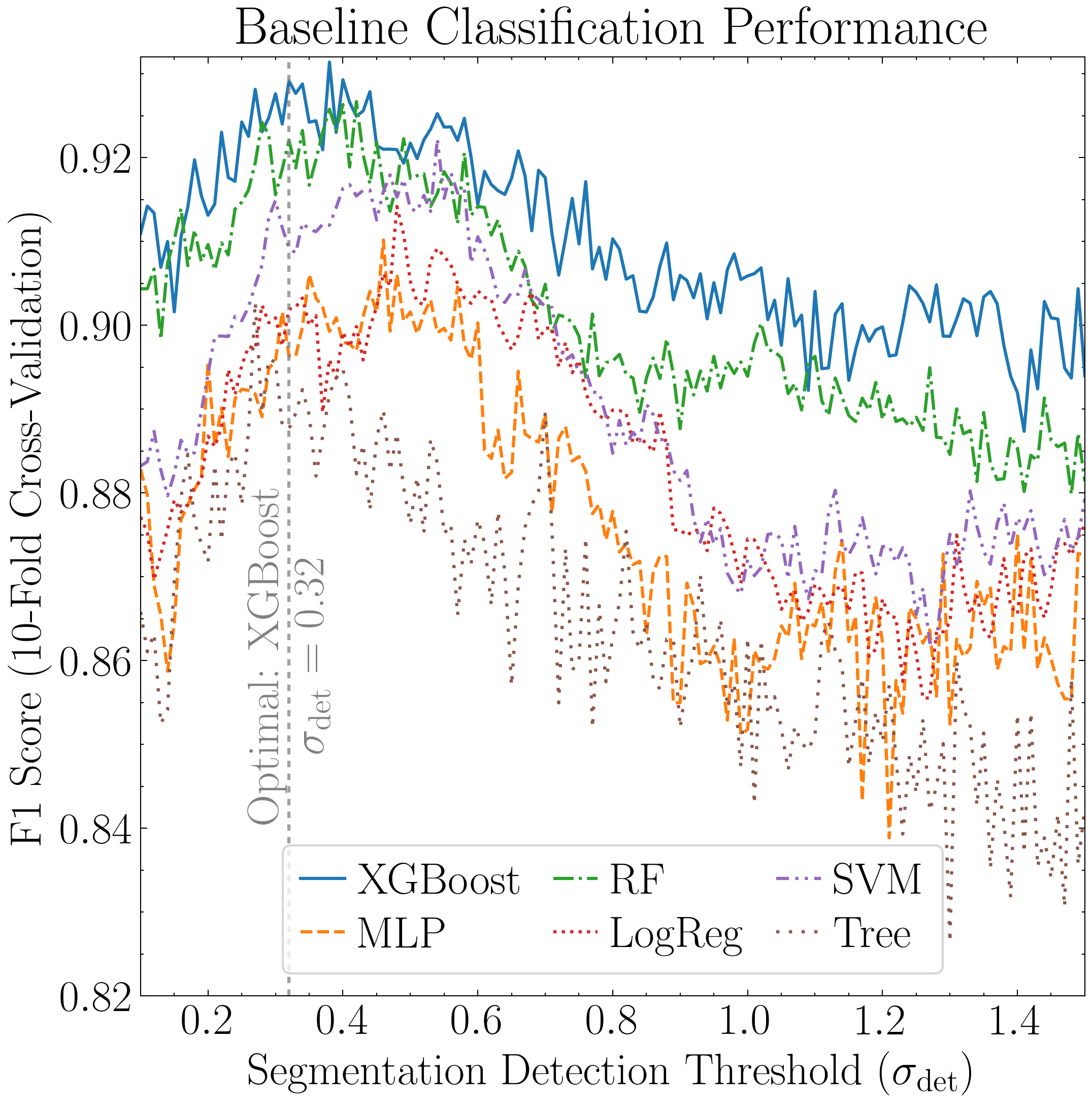
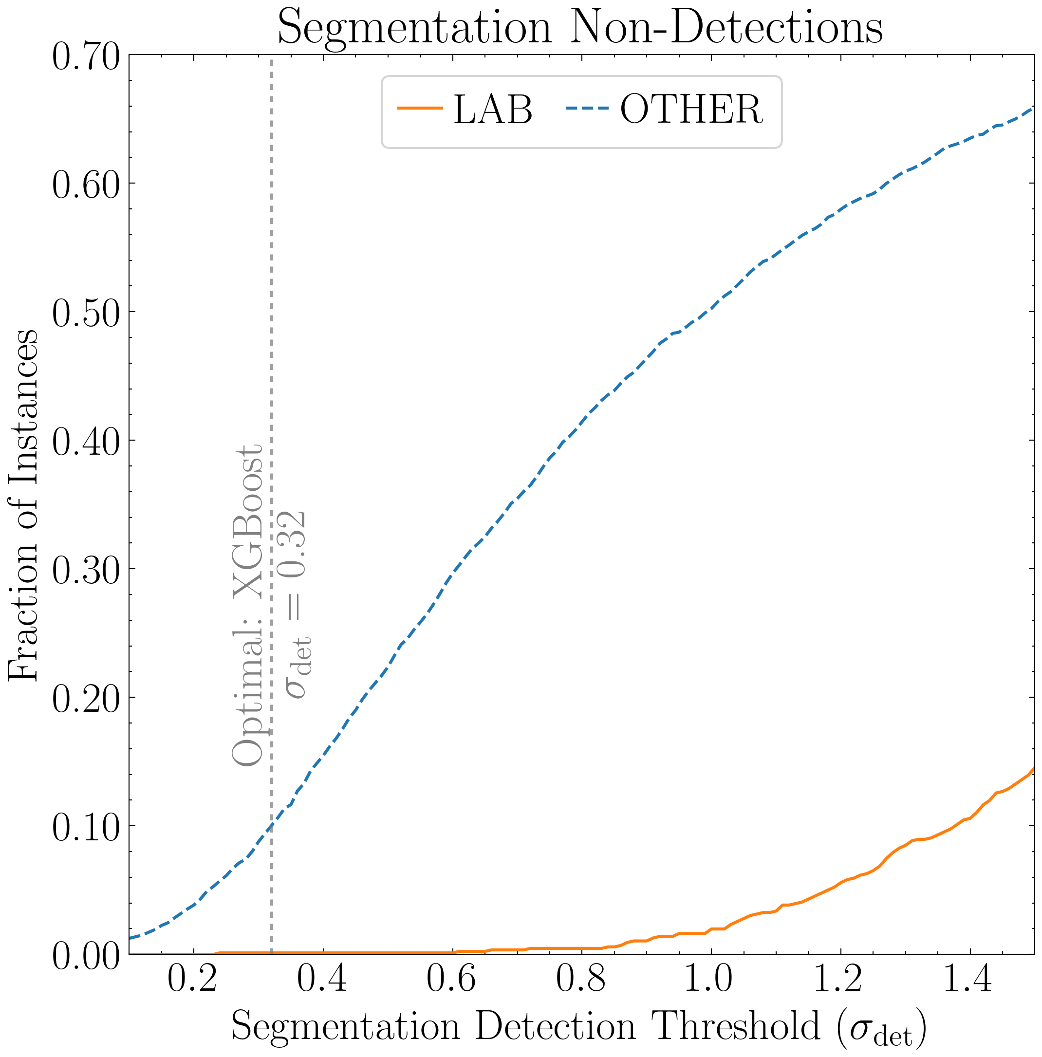
With these files, we can now plot the non-detections and evaluate performance as a function of the detection threshold.
import numpy as np
import pandas as pd
import matplotlib.pyplot as plt
from matplotlib.ticker import FuncFormatter
from matplotlib.lines import Line2D
import scienceplots
plt.style.use('science')
plt.rcParams.update({'font.size': 21, 'lines.linewidth':1.5})

# Load the data saved in previous script
df_metrics = pd.read_csv('baseline_classifiers.csv')
non_detect_data = np.loadtxt('non_detections_Bw')

# Query best classifier according to the F1 score at chosen sigma
metric = 'f1'
best_sigma = 0.32  # The highest F1 score is at sigma=0.38 but comparable at 0.32 which yields more detections
subdf = df_metrics[df_metrics['nsig'] == best_sigma]
chosen_row = subdf[subdf[metric] == subdf[metric].max()].iloc[0]
best_clf = chosen_row['classifier']
best_f1 = chosen_row[metric]

# Plots
fig1, ax1 = plt.subplots(figsize=(8, 8))

# Line styles
colors = plt.cm.tab10.colors
linestyles = ['-', '--', '-.', ':', (0, (4, 2, 1, 2, 1, 2)), (0, (1, 3))]

# The classifiers in order so they show from best to worst in legend (top left to bottom right)
clf_order = ['xgb', 'nn', 'rf', 'logreg', 'svc', 'tree']
clf_display = {'xgb': 'XGBoost', 'nn': 'MLP', 'rf': 'RF', 'logreg': 'LogReg', 'svc': 'SVC', 'tree': 'Tree'}

for i, clf in enumerate(clf_order):
    subdf = df_metrics[df_metrics['classifier'] == clf]
    ax1.plot(subdf['nsig'], subdf[metric], label=clf_display[clf], color=colors[i % 10], linestyle=linestyles[i % len(linestyles)])

# Highlight the optimal detection threshold
ax1.axvline(best_sigma, linestyle=(0, (2, 2)), alpha=0.75, color='gray')
ax1.annotate(f'Optimal: {clf_display[best_clf]}\n' + r'$\sigma_{\rm det}$ = ' + f'{best_sigma:.2f}',
    xy=(best_sigma, 0.881),
    xytext=(0.47, 0),
    textcoords='offset points',
    ha='center', va='top',
    color='gray', rotation=90)

ax1.set_title('Baseline Classification Performance')
ax1.set_xlabel(r'Segmentation Detection Threshold ($\sigma_{\rm det}$)')
ax1.set_ylabel('F1 Score (10-Fold Cross-Validation)')
ax1.set_xlim((0.1, 1.5)); ax1.set_ylim(0.82, 0.932)
ax1.legend(loc='lower center', ncol=3, handlelength=1, handletextpad=0.3, columnspacing=0.7, labelspacing=0.3, frameon=True, fancybox=True)
fig1.savefig('nsigs_f1_all_classifiers.png', dpi=300, bbox_inches='tight')
plt.show()

# Plot the non-detections
fig2, ax2 = plt.subplots(figsize=(8, 8))

lns1, = ax2.plot(non_detect_data[:, 0], non_detect_data[:, 2], linestyle='--', label='OTHER', color='tab:blue')
lns2, = ax2.plot(non_detect_data[:, 0], non_detect_data[:, 1], linestyle='-', label='LAB', color='tab:orange')

ax2.axvline(best_sigma, linestyle=(0, (2, 2)), alpha=0.75, color='gray')
ax2.annotate(f'Optimal: {clf_display[best_clf]}\n' + r'$\sigma_{\rm det}$ = ' + f'{best_sigma:.2f}',
    xy=(best_sigma, 0.4),
    xytext=(0.47, 0),
    textcoords='offset points',
    ha='center', va='top',
    color='gray', rotation=90)

ax2.legend(handles=[lns2, lns1], labels=['LAB', 'OTHER'], loc='upper center', ncol=2, handlelength=1,  handletextpad=0.3, columnspacing=0.7, labelspacing=0.3, frameon=True, fancybox=True)

ax2.set_title('Segmentation Non-Detections')
ax2.set_xlabel(r'Segmentation Detection Threshold ($\sigma_{\rm det}$)')
ax2.set_ylabel('Fraction of Instances')
ax2.set_xlim((0.1, 1.5)); ax2.set_ylim(0, 0.7)
ax2.yaxis.set_major_formatter(FuncFormatter(lambda x, _: f'{x:.2f}'))

fig2.savefig('nsigs_normalized_non_detections.png', dpi=300, bbox_inches='tight')
plt.show()
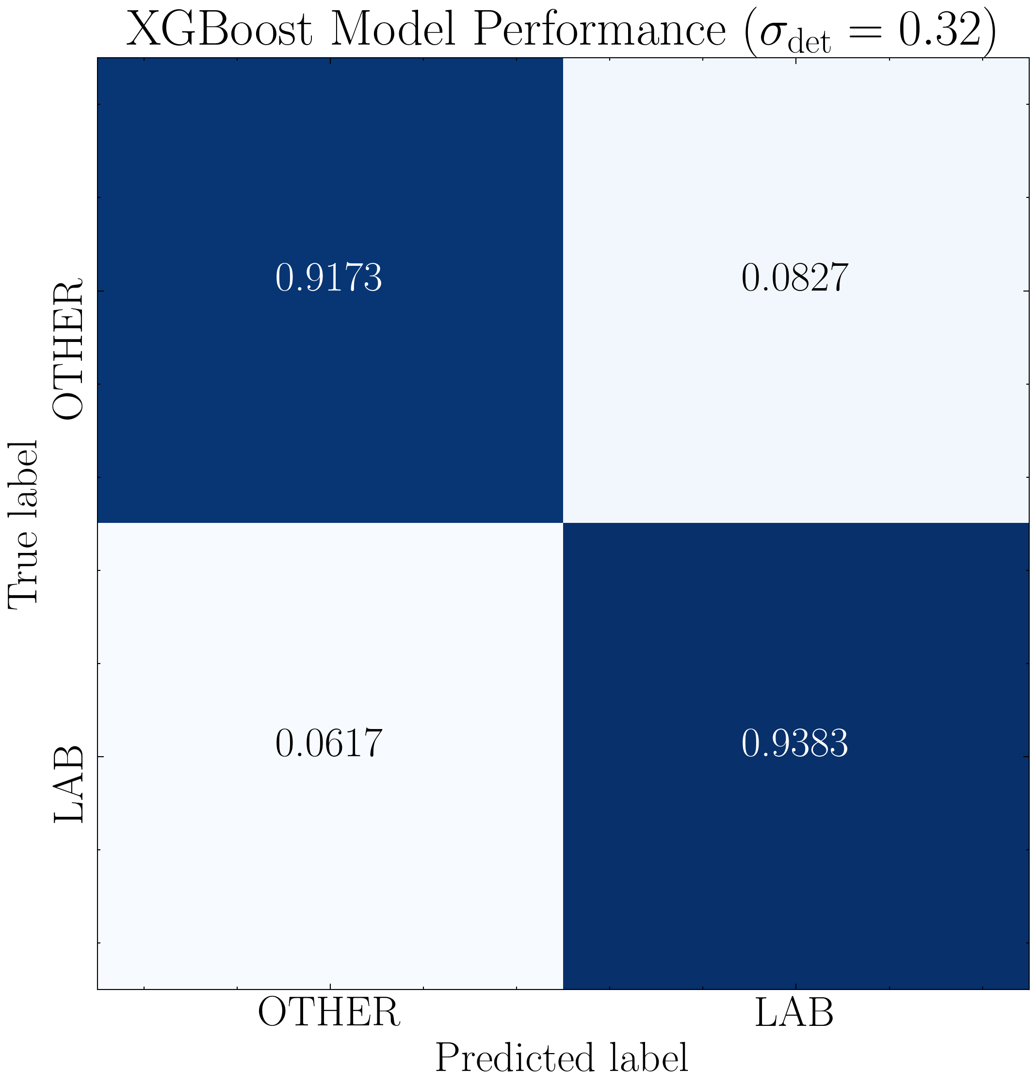
Baseline XGBoost Model
We now re-train the optimal XGBoost model using the best-performing detection threshold of 0.32 and plot the resulting confusion matrix using the ensemble_model module.
import numpy as np
import pandas as pd
from pyBIA import ensemble_model, data_processing

# Where the training set files were saved
nsig_path = 'nsigs/'

sig = 0.32 #The optimal sig threshold to apply as per Figure 2
df = pd.read_csv(f'{nsig_path}_Bw_training_set_nsig_{sig}')

# Log-transform the Hu moments
hu_cols = ['Hu1', 'Hu2', 'Hu3', 'Hu4', 'Hu5', 'Hu6', 'Hu7']
df[hu_cols] = df[hu_cols].apply(data_processing.signed_log_transform)

# Omit any non-detections (nan mags (~10%) and nan Hu moments (~0.02%))
mask = np.where((df['area'] != -999) & np.isfinite(df['mag']) & np.all(np.isfinite(df[[f'Hu{i}' for i in range(1, 8)]]), axis=1))[0]

# Balance both classes to be of same size
blob_index = np.where(df['flag'].iloc[mask] == 1)[0]
other_index = np.where(df['flag'].iloc[mask] == 0)[0]
df_filtered = df.iloc[mask[np.concatenate((blob_index, other_index[:len(blob_index)]))]]

#These are the features to use, note that the catalog includes more than this!
columns = [
    'mag', 'mag_err',
    'M00', 'M10', 'M01', 'M20', 'M11', 'M02', 'M30', 'M21', 'M12', 'M03',
    'mu20', 'mu11', 'mu02', 'mu30', 'mu21', 'mu12', 'mu03',
    'G10', 'G01', 'G20', 'G11', 'G02', 'G30', 'G21', 'G12', 'G03',
    'Hu1', 'Hu2', 'Hu3', 'Hu4', 'Hu5', 'Hu6', 'Hu7',
    'L00', 'L10', 'L01', 'L20', 'L11', 'L02', 'L30', 'L21', 'L12', 'L03',
    'area', 'covar_sigx2', 'covar_sigy2', 'covar_sigxy', 'covariance_eigval1', 'covariance_eigval2',
    'cxx', 'cxy', 'cyy', 'eccentricity', 'ellipticity', 'elongation',
    'equivalent_radius', 'fwhm', 'gini', 'orientation', 'perimeter',
    'semimajor_sigma', 'semiminor_sigma', 'max_value', 'min_value'
]

# Training data arrays
data_x, data_y = np.array(df_filtered[columns]), np.array(df_filtered['flag'])

# Classifier object
SEED_NO = 1909 # Seed No for shuffling the data when assessing the classifier
impute = False # No need to impute, no NaN should be present
optimize = False # Disabling optimization routine, this is the baseline model
opt_cv = 10 # Will assess performance using 10Fold CV
clf = 'xgb' # Will train an XGBoost model (optimal model)

model = ensemble_model.Classifier(
        data_x,
        data_y,
        clf=clf,
        impute=impute,
        optimize=optimize,
        opt_cv=opt_cv,
        SEED_NO=SEED_NO
        )

model.create()

# Plot confusion matrix with text class labels (instead of numerical) for the confusion matrix
data_y_labels = ['LAB' if i == 1 else 'OTHER' for i in data_y]
model.plot_conf_matrix(data_y=data_y_labels, title=r'XGBoost Model Performance ($\sigma_{\rm det} = 0.32$)', savefig=True)
Optimized XGBoost Models
We now proceed with the generated training set at the optimal detection threshold. Whereas the previous analysis trained baseline models, this step invokes our optimization routine to select the most informative features and the best hyperparameters for the XGBoost engine. In the code below, two distinct models are optimized: one using the ``boruta_model``=”rf” option and another using the “xgb” option, which applies a more conservative feature-selection approach. This is all done using the ensemble_model module.
import numpy as np
import pandas as pd
from pyBIA import ensemble_model, data_processing

# Where the training set files were saved
nsig_path = 'nsigs/'

sig = 0.32 #The optimal sig threshold to apply as per Figure 2
df = pd.read_csv(f'{nsig_path}_Bw_training_set_nsig_{sig}')
hu_cols = ['Hu1', 'Hu2', 'Hu3', 'Hu4', 'Hu5', 'Hu6', 'Hu7']
df[hu_cols] = df[hu_cols].apply(data_processing.signed_log_transform)

# Omit any non-detections
mask = np.where((df['area'] != -999) & np.isfinite(df['mag']) & np.all(np.isfinite(df[[f'Hu{i}' for i in range(1, 8)]]), axis=1))[0]

# Balance both classes to be of same size
blob_index = np.where(df['flag'].iloc[mask] == 1)[0]
other_index = np.where(df['flag'].iloc[mask] == 0)[0]
df_filtered = df.iloc[mask[np.concatenate((blob_index, other_index[:len(blob_index)]))]]

#These are the features to use, note that the catalog includes more than this!
columns = [
    'mag', 'mag_err',
    'M00', 'M10', 'M01', 'M20', 'M11', 'M02', 'M30', 'M21', 'M12', 'M03',
    'mu20', 'mu11', 'mu02', 'mu30', 'mu21', 'mu12', 'mu03',
    'G10', 'G01', 'G20', 'G11', 'G02', 'G30', 'G21', 'G12', 'G03',
    'Hu1', 'Hu2', 'Hu3', 'Hu4', 'Hu5', 'Hu6', 'Hu7',
    'L00', 'L10', 'L01', 'L20', 'L11', 'L02', 'L30', 'L21', 'L12', 'L03',
    'area', 'covar_sigx2', 'covar_sigy2', 'covar_sigxy', 'covariance_eigval1', 'covariance_eigval2',
    'cxx', 'cxy', 'cyy', 'eccentricity', 'ellipticity', 'elongation',
    'equivalent_radius', 'fwhm', 'gini', 'orientation', 'perimeter',
    'semimajor_sigma', 'semiminor_sigma', 'max_value', 'min_value'
]

# Training data arrays
data_x, data_y = np.array(df_filtered[columns]), np.array(df_filtered['flag'])

# Will run the optimization routine all at once, feature selection first followed by engine hyperparameter optimization
# Enabling 10-fold cross validation which increases the hyperparameter optimization time ten-fold

# XGB-BASED BorutaSHAP
SEED_NO = 1909 # The seed number that will initialize the stochastic process (e.g., model training)
clf = 'xgb' # The classification model that will be trined, options are: 'xgb', 'rf' and 'nn'
impute = False # Whether to impute missing values (NaN)
optimize = True # Will enable the optimization routine
scoring_metric = 'f1' # The optimization trials will be assessed according to the F1 Score
opt_cv = 10 # The number of folds to perform during cross validation, ONLY used during optimization (`optimize`=True)
boruta_trials = 100 # Number of feature selection trials to perform (This is fast especially with `boruta_model`='xgb')
boruta_model = 'xgb' # The model to use when assessing feautre importances during feature selection (either 'rf' or 'xgb', DOES NOT have to match the `clf`)
n_iter = 100 # Number of hyperparameter optimization trials to perform, can set to 0 to disable hyperparam tuning
limit_search = True # Set to False to expand the hyperparameter search space (will take longer)

# Instantiate the Classifier
model = ensemble_model.Classifier(
        data_x,
        data_y,
        clf=clf,
        impute=impute,
        optimize=optimize,
        boruta_trials=boruta_trials,
        boruta_model=boruta_model,
        n_iter=n_iter,
        scoring_metric=scoring_metric,
        opt_cv=opt_cv,
        limit_search=limit_search,
        SEED_NO=SEED_NO
        )

# Tune and train the model
model.create()

# Save the model
model.save(dirname=f'ensemble_model_xgb_boruta_{boruta_model}')

boruta_model = 'rf' # Change to RF-based feature importance ranking during optimization

# RF-BASED BorutaSHAP
model = ensemble_model.Classifier(
        data_x,
        data_y,
        clf=clf,
        impute=impute,
        optimize=optimize,
        boruta_trials=boruta_trials,
        boruta_model=boruta_model,
        n_iter=n_iter,
        scoring_metric=scoring_metric,
        opt_cv=opt_cv,
        limit_search=limit_search,
        SEED_NO=SEED_NO
        )

model.create()
model.save(dirname=f'ensemble_model_xgb_boruta_{boruta_model}')
The XGBoost model optimized with RF-based feature importance (for computing SHAP values) can be downloaded here.
The XGBoost model optimized with XGBoost-based feature importance (for computing SHAP values) can be downloaded here.
NOTE: These models were saved using Python 3.12. To avoid pickle dependency issues, please load them using Python 3.12.
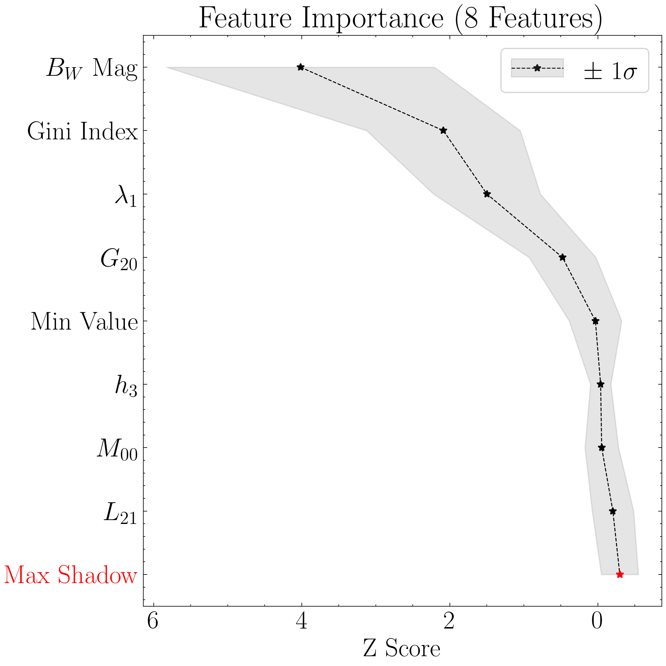
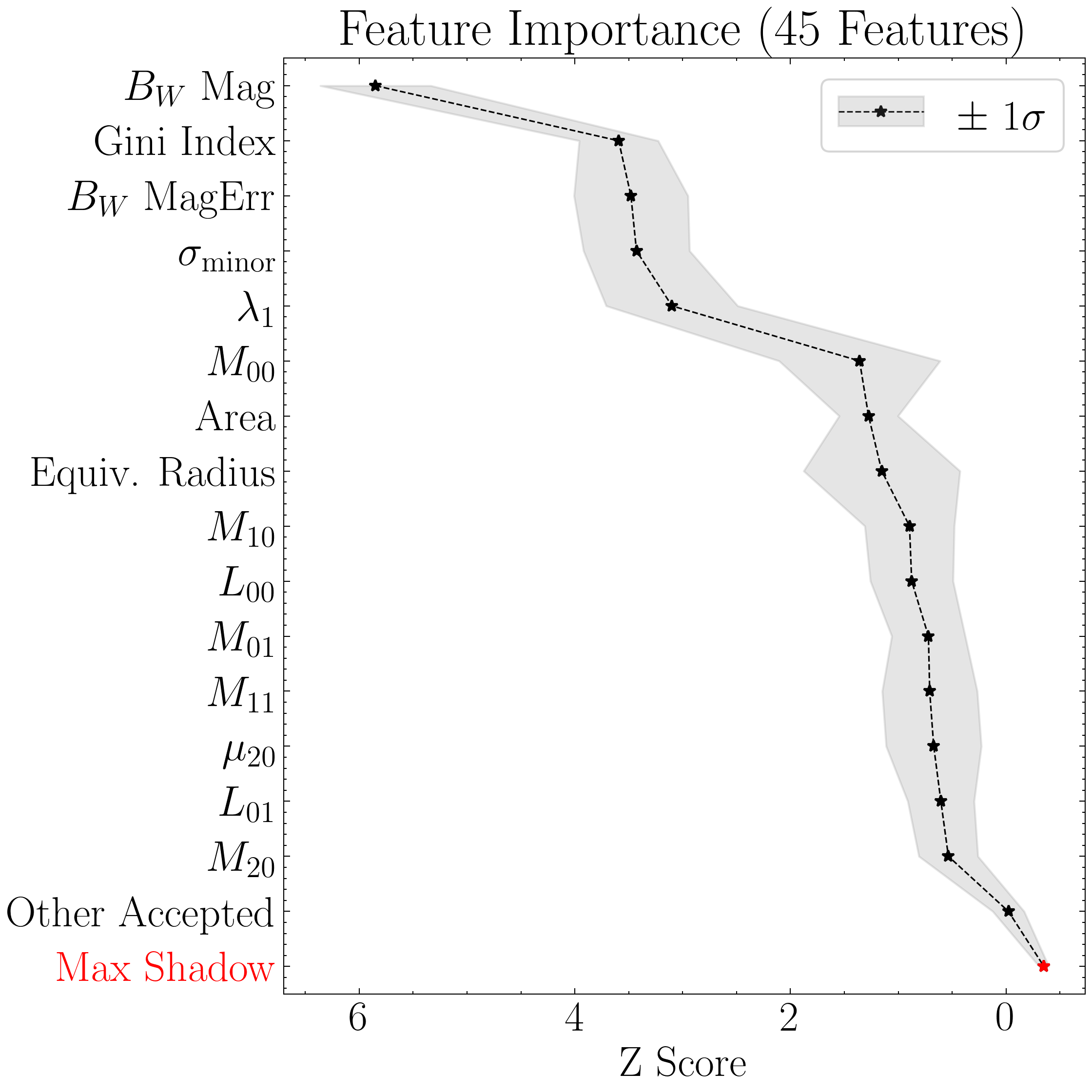
Below, we plot the optimization results (feature-selection from the BorutaSHAP algorithm and the subsequent Optuna-based hyperparameter optimization) using the built-in class methods.
import numpy as np
from pyBIA import ensemble_model, data_processing
import pandas as pd
# Where the training set files were saved
nsig_path = 'nsigs/'
sig = 0.32 #The optimal sig threshold to apply as per Figure 2
df = pd.read_csv(f'{nsig_path}_Bw_training_set_nsig_{sig}')
# Log-transform the Hu moments
hu_cols = ['Hu1', 'Hu2', 'Hu3', 'Hu4', 'Hu5', 'Hu6', 'Hu7']
df[hu_cols] = df[hu_cols].apply(data_processing.signed_log_transform)
# Omit any non-detections (nan mags (~10%) and nan Hu moments (~0.02%))
mask = np.where((df['area'] != -999) & np.isfinite(df['mag']) & np.all(np.isfinite(df[[f'Hu{i}' for i in range(1, 8)]]), axis=1))[0]
# Balance both classes to be of same size
blob_index = np.where(df['flag'].iloc[mask] == 1)[0]
other_index = np.where(df['flag'].iloc[mask] == 0)[0]
df_filtered = df.iloc[mask[np.concatenate((blob_index, other_index[:len(blob_index)]))]]
#These are the features to use, note that the catalog includes more than this!
columns = [
'mag', 'mag_err',
'M00', 'M10', 'M01', 'M20', 'M11', 'M02', 'M30', 'M21', 'M12', 'M03',
'mu20', 'mu11', 'mu02', 'mu30', 'mu21', 'mu12', 'mu03',
'G10', 'G01', 'G20', 'G11', 'G02', 'G30', 'G21', 'G12', 'G03',
'Hu1', 'Hu2', 'Hu3', 'Hu4', 'Hu5', 'Hu6', 'Hu7',
'L00', 'L10', 'L01', 'L20', 'L11', 'L02', 'L30', 'L21', 'L12', 'L03',
'area', 'covar_sigx2', 'covar_sigy2', 'covar_sigxy', 'covariance_eigval1', 'covariance_eigval2',
'cxx', 'cxy', 'cyy', 'eccentricity', 'ellipticity', 'elongation',
'equivalent_radius', 'fwhm', 'gini', 'orientation', 'perimeter',
'semimajor_sigma', 'semiminor_sigma', 'max_value', 'min_value'
]
# Training data arrays
data_x, data_y = np.array(df_filtered[columns]), np.array(df_filtered['flag'])
#LOAD THE SAVED MODELS AND PLOT THE OPTIMIZATION RESULTS
#XGB-Based BorutaSHAP
clf = 'xgb' # The classification model
impute = False # Will not impute NaN values, as they should not be present after masking non-detections
# Instantiate the classifier and load the saved model
# First load the model that was optimized using XGBoost-based feature selection (8 features selected)
xgboost8_model = ensemble_model.Classifier(data_x, data_y, clf=clf, impute=impute)
xgboost8_model.load('ensemble_model_xgb_boruta_xgb')
# Next load the model that was optimized using RF-based feature selection (45 features selected)
xgboost45_model = ensemble_model.Classifier(data_x, data_y, clf=clf, impute=impute)
xgboost45_model.load('ensemble_model_xgb_boruta_rf')
# Plot the feature selection results
#Setting custom column names for plotting purposes
columns_formatted = [
r'$B_W$ Mag', r'$B_W$ MagErr',
r'$M_{00}$', r'$M_{10}$', r'$M_{01}$', r'$M_{20}$', r'$M_{11}$', r'$M_{02}$', r'$M_{30}$', r'$M_{21}$', r'$M_{12}$', r'$M_{03}$',
r'$\mu_{20}$', r'$\mu_{11}$', r'$\mu_{02}$', r'$\mu_{30}$', r'$\mu_{21}$', r'$\mu_{12}$', r'$\mu_{03}$',
r'$G_{10}$', r'$G_{01}$', r'$G_{20}$', r'$G_{11}$', r'$G_{02}$', r'$G_{30}$', r'$G_{21}$', r'$G_{12}$', r'$G_{03}$',
r'$h_1$', r'$h_2$', r'$h_3$', r'$h_4$', r'$h_5$', r'$h_6$', r'$h_7$',
r'$L_{00}$', r'$L_{10}$', r'$L_{01}$', r'$L_{20}$', r'$L_{11}$', r'$L_{02}$', r'$L_{30}$', r'$L_{21}$', r'$L_{12}$', r'$L_{03}$',
'Area', r'$\sigma^2(x)$', r'$\sigma^2(y)$', r'$\sigma^2(xy)$', r'$\lambda_1$', r'$\lambda_2$', r'$C_{xx}$', r'$C_{xy}$', r'$C_{yy}$',
'Eccentricity', 'Ellipticity', 'Elongation', 'Equiv. Radius', 'FWHM', 'Gini Index', 'Orientation', 'Perimeter',
r'$\sigma_{\rm major}$', r'$\sigma_{\rm minor}$', 'Max Value', 'Min Value'
]
top = 'all' # Will show all accepted features
include_other = True # The other accepted will be shown as a single point (combined Z-Scores)
include_shadow = True # Whether to include a 'random performance' benchmark (i.e., the "shadow" feature)
include_rejected = False # Whether to show the features that were not deemed important
flip_axes = True # Set to False to plot the features on the x-axis (if you're plotting a lot of them)
title = 'Feature Importance (8 Features)' # Figure title
save_data = False # Whether to save the feature importances to a csv file
savefig = False # Whether to save the figure (note that current version of program always saves with same figname so careful with overwrites)
# First plot the XGBoost-based feature selection results
xgboost8_model.plot_feature_opt(
feat_names=columns_formatted,
top=top,
include_other=include_other,
include_shadow=include_shadow,
include_rejected=include_rejected,
flip_axes=flip_axes,
save_data=save_data,
title=title,
savefig=savefig
)
# Next plot the RF-based feature selection results
top = 15 # Only plot the top 15 accepted features
title = 'Feature Importance (45 Features)' # Figure title
xgboost45_model.plot_feature_opt(
feat_names=columns_formatted,
top=top,
include_other=include_other,
include_shadow=include_shadow,
include_rejected=include_rejected,
flip_axes=flip_axes,
save_data=save_data,
title=title,
savefig=savefig
)
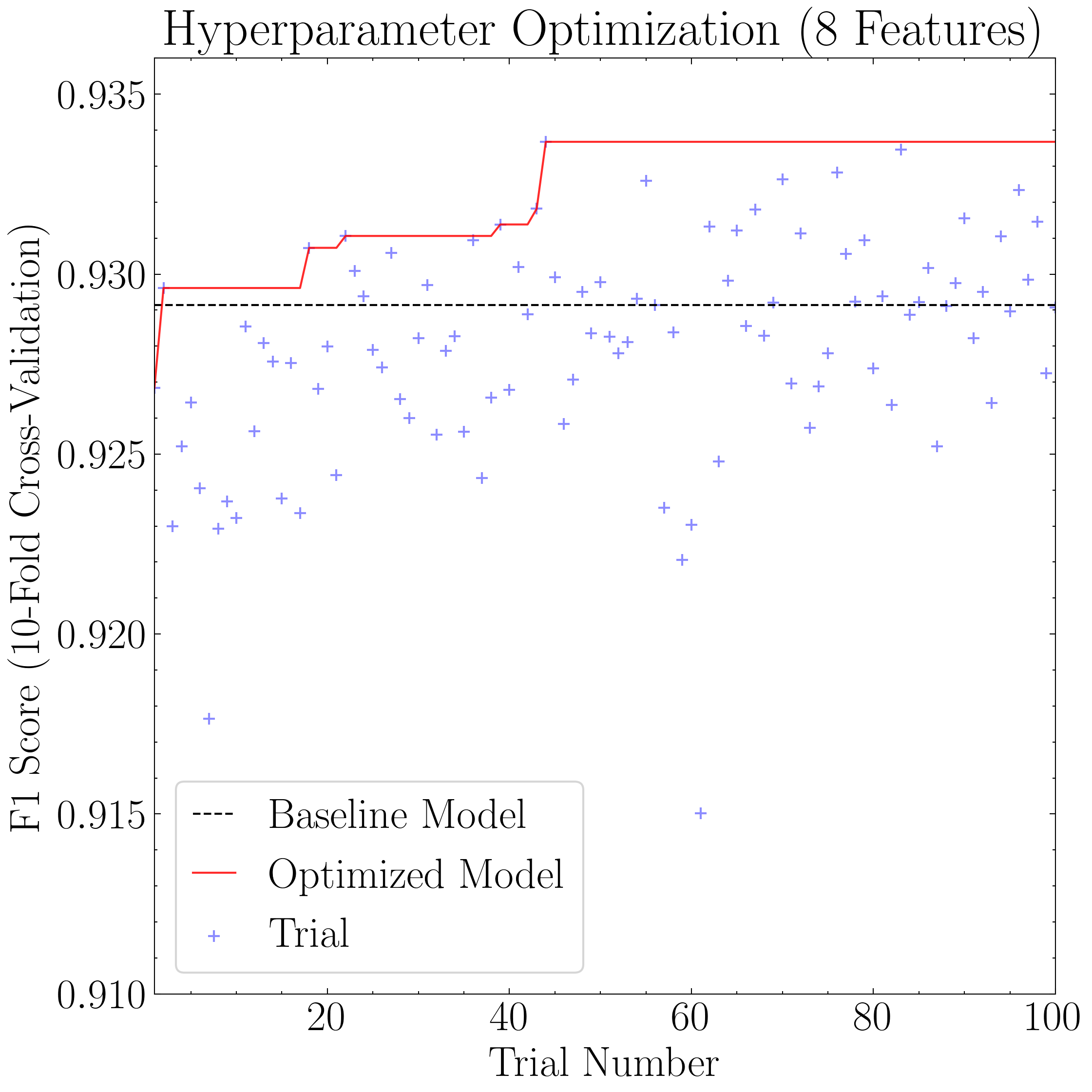
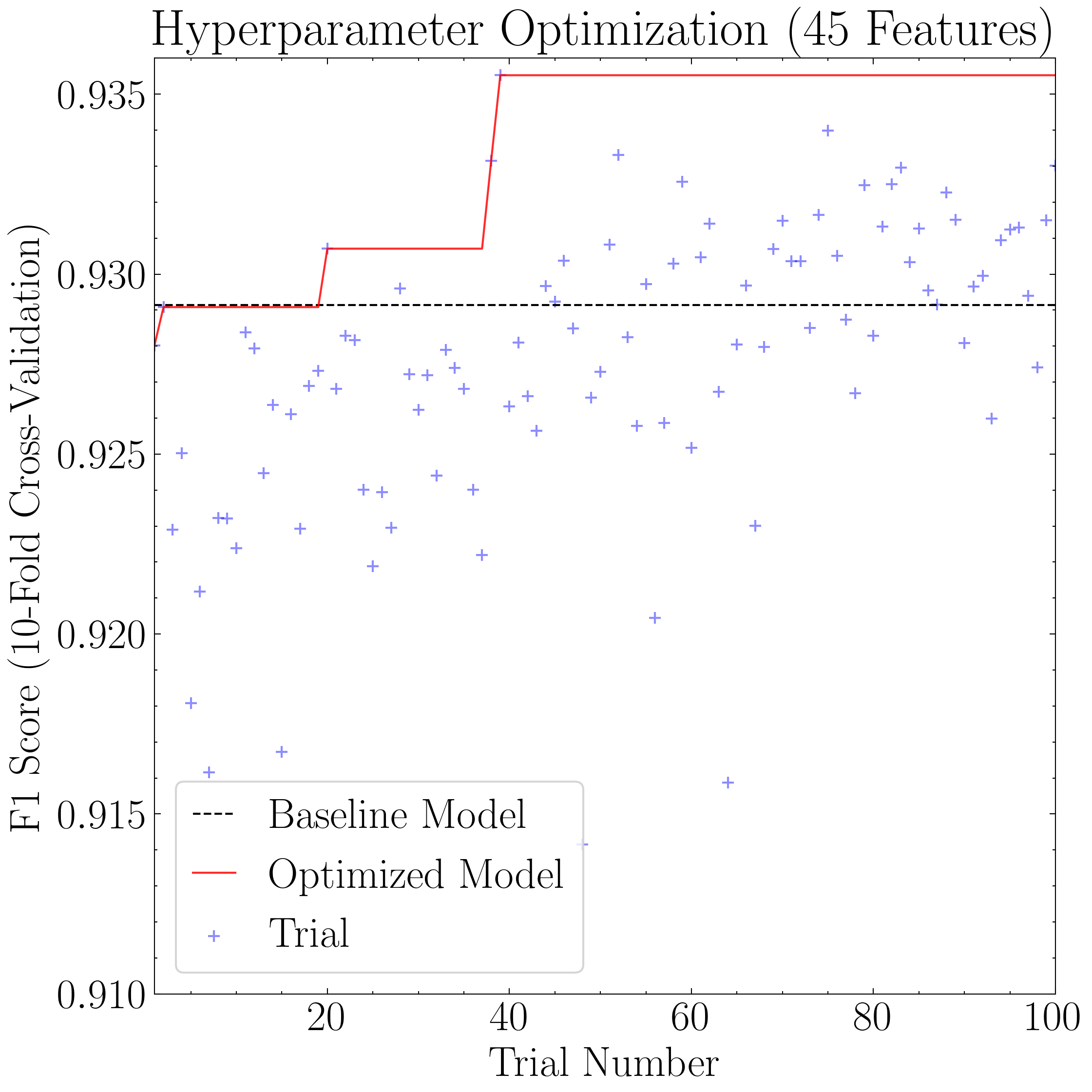
# Plot the hyperparameter optimization results
baseline = 0.92914 # The maximum XGBoost baseline accuracy as per Figure 2
xlim = (1, 100) # xlim axes
ylim = (0.91, 0.936) # ylim axes
xlog = False # Whether to log-scale x-axis
ylog = False # Whether to log-scale y-axis
ylabel = 'F1 Score (10-Fold Cross-Validation)'
loc = 'lower left' # Legend location
ncol = 1 # No of columns in legend
savefig = True # Whether to save the figure (note that current version of program always saves with same figname so careful about overwrites)
# First plot the results from the XGBoost model trained with 8 features
title = 'Hyperparameter Optimization (8 Features)' # Fig title
xgboost8_model.plot_hyper_opt(
baseline=baseline,
xlim=xlim,
ylim=ylim,
xlog=xlog,
ylog=ylog,
title=title,
ylabel=ylabel,
loc=loc,
ncol=ncol,
savefig=savefig
)
# First plot the results from the XGBoost model trained with 45 features
title = 'Hyperparameter Optimization (45 Features)' # Fig title
xgboost45_model.plot_hyper_opt(
baseline=baseline,
xlim=xlim,
ylim=ylim,
xlog=xlog,
ylog=ylog,
ylabel=ylabel,
title=title,
loc=loc,
ncol=ncol,
savefig=savefig
)
Boötes Morphological Catalog
With the optimal models saved, we now extract features for all 2 million OTHER objects in the dataset using the Catalog class. The positional catalog information for these objects is compiled in the following dataframe: Other_Objects_Catalog.
Using this file, we can construct a catalog for the entire dataset to run the XGBoost classification (excluding the 866 LAB objects from the provided training set).
import os
import numpy as np
import pandas as pd
from astropy.io import fits
from pyBIA import catalog

other_catalog = pd.read_csv('Other_Objects_Catalog.csv')

data_path = 'NDWFS/fits_images/Bw_FITS/'
data_error_path = 'NDWFS_Bootes/Error_Maps/Bw/'

sig = 0.32 # The optimal noise-detection threshold to apply

# Loop through all the fields and save the field catalogs to avoid memory issues
counter = 0
for fieldname in np.unique(np.array(other_catalog['field_name'])):
        counter += 1
        print(fieldname, f'{counter} out of 27')
        # Load the field data
        data_hdu, error_map = fits.open(data_path+fieldname+'_Bw_03_fix.fits'), fits.getdata(data_error_path+fieldname+'_Bw_03_rms.fits.fz')
        # Extract the data and corresponding ZP and exptime
        data_map, zeropoint, exptime = data_hdu[0].data, data_hdu[0].header['MAGZERO'], data_hdu[0].header['EXPTIME']
        # Select only the samples from this subfield
        subfield_index = np.where(other_catalog['field_name']==fieldname)[0]
        xpix, ypix = other_catalog[['xpix', 'ypix']].iloc[subfield_index].values.T
        objname, field, flag = other_catalog[['obj_name', 'field_name', 'flag']].iloc[subfield_index].values.T
        # Create the catalog object
        cat = catalog.Catalog(
                data_map,
                error=error_map,
                x=xpix,
                y=ypix,
                zp=zeropoint,
                exptime=exptime,
                nsig=sig,
                flag=flag,
                obj_name=objname,
                field_name=field,
                invert=True) # Invert is used to flip x/y coordinates, for ease in handling standard .fits coord system
        # Generate the catalog and save the subfield catalog, after which it is appended to the master frame
        cat.create(save_file=True, filename='Cat_BW_Subfield_'+fieldname)

# Now load each subfield individually and create one master catalog
fnames = [i for i in os.listdir() if 'Cat_BW_Subfield_' in i]

frame = [] #To store all 27 subfields
for fname in fnames:
        cat = pd.read_csv(fname)
        frame.append(cat)

# Combine all 27 sub-catalogs into one master frame and save
frame = pd.concat(frame, axis=0, join='inner')
frame.to_csv(f'Other_Catalog_Master_{sig}', chunksize=1000)
The master catalog generated above is available for download here.
Using this catalog, we can now load the optimal models to generate predictions. Predictions will be produced with both the baseline and optimal models to compare the resulting probability distributions.
Predictions & LOO CV
In the following script, we perform model predictions on the entire NDWFS Boötes field to generate the candidate catalogs (i.e., sources with probability predictions greater than or equal to 0.5).
These candidate catalogs exclude the 866 LAB training objects, which were deliberately removed from the source catalog. While the randomly selected objects that comprised the OTHER class remain in the catalog, they were used for training purposes and thus cannot be fairly assessed, as their presence as OTHER training instances skews their probability predictions. We thus employ a leave-one-out cross-validation (LOO CV) routine to fairly assess both the LAB and OTHER training set instances.
import numpy as np
import numpy as np
import pandas as pd
from pyBIA import ensemble_model, data_processing

# Load all 2 million catalog objects and create a sub-catalog of LAB candidates #
# LoO Analysis is performed on the training data in order to determine which of these sources would be considered new candidates

# Where the training set files were saved
nsig_path = 'nsigs/'

# First load the training data
sig = 0.32 #The optimal sig threshold to apply as per Figure 2
df = pd.read_csv(f'{nsig_path}_Bw_training_set_nsig_{sig}')

# Log-transform the Hu moments
hu_cols = ['Hu1', 'Hu2', 'Hu3', 'Hu4', 'Hu5', 'Hu6', 'Hu7']
df[hu_cols] = df[hu_cols].apply(data_processing.signed_log_transform)

# Omit any non-detections (nan mags (~10%) and nan Hu moments (~0.02%))
mask = np.where((df['area'] != -999) & np.isfinite(df['mag']) & np.all(np.isfinite(df[[f'Hu{i}' for i in range(1, 8)]]), axis=1))[0]

# Balance both classes to be of same size
blob_index = np.where(df['flag'].iloc[mask] == 1)[0]
other_index = np.where(df['flag'].iloc[mask] == 0)[0]
df_filtered = df.iloc[mask[np.concatenate((blob_index, other_index[:len(blob_index)]))]]

#These are the features to use, note that the catalog includes more than this!
columns = [
    'mag', 'mag_err',
    'M00', 'M10', 'M01', 'M20', 'M11', 'M02', 'M30', 'M21', 'M12', 'M03',
    'mu20', 'mu11', 'mu02', 'mu30', 'mu21', 'mu12', 'mu03',
    'G10', 'G01', 'G20', 'G11', 'G02', 'G30', 'G21', 'G12', 'G03',
    'Hu1', 'Hu2', 'Hu3', 'Hu4', 'Hu5', 'Hu6', 'Hu7',
    'L00', 'L10', 'L01', 'L20', 'L11', 'L02', 'L30', 'L21', 'L12', 'L03',
    'area', 'covar_sigx2', 'covar_sigy2', 'covar_sigxy', 'covariance_eigval1', 'covariance_eigval2',
    'cxx', 'cxy', 'cyy', 'eccentricity', 'ellipticity', 'elongation',
    'equivalent_radius', 'fwhm', 'gini', 'orientation', 'perimeter',
    'semimajor_sigma', 'semiminor_sigma', 'max_value', 'min_value'
]

# Training data arrays
data_x, data_y = np.array(df_filtered[columns]), np.array(df_filtered['flag'])

clf = 'xgb' # The classification model
impute = False # Will not impute NaN values, as they should not be present after masking non-detections

# This is the base model, no hyperparameter optimization, uses all the features
base_model = ensemble_model.Classifier(data_x, data_y, clf=clf, impute=impute)
base_model.create()

# These are the optimized models
xgboost_8_model = ensemble_model.Classifier(data_x, data_y, clf=clf, impute=impute)
xgboost_8_model.load('ensemble_model_xgb_boruta_xgb')

xgboost_45_model = ensemble_model.Classifier(data_x, data_y, clf=clf, impute=impute)
xgboost_45_model.load('ensemble_model_xgb_boruta_rf')

# Load the catalog containing all 2 million other objects, extracted using sig=0.32
other_all = pd.read_csv('Other_Catalog_Master_0.32')

# Remove the 859 OTHER objects that are present in the training set, we will assess these individually using LoO
other_all = other_all[~other_all['obj_name'].isin(df_filtered['obj_name'])]

# Log transform the Hu moments
other_all[hu_cols] = other_all[hu_cols].apply(data_processing.signed_log_transform)

# Omit non-detections
mask = np.where((other_all['area'] != -999) & np.isfinite(other_all['mag']) & np.all(np.isfinite(other_all[[f'Hu{i}' for i in range(1, 8)]]), axis=1))[0]

other_all = other_all.iloc[mask]

# Create the data_x array
other_data_x = np.array(other_all[columns])

# Predict all samples to create a candidates catalog
predictions_base_model = base_model.predict(other_data_x)
predictions_xgboost_8 = xgboost_8_model.predict(other_data_x)
predictions_xgboost_45 = xgboost_45_model.predict(other_data_x)

# Select LAB detections (flag = 1)
index_base = np.where(predictions_base_model[:,0] == 1)[0]
index_xgboost_8 = np.where(predictions_xgboost_8[:,0] == 1)[0]
index_xgboost_45 = np.where(predictions_xgboost_45[:,0] == 1)[0]

# Index the catalog to select only the positive detections
candidate_catalog_base = other_all.iloc[index_base]
candidate_catalog_xgboost_8 = other_all.iloc[index_xgboost_8]
candidate_catalog_xgboost_45 = other_all.iloc[index_xgboost_45]

# Save the probability predictions as a new columns
candidate_catalog_base['proba'] = predictions_base_model[index_base][:,1]
candidate_catalog_xgboost_8['proba'] = predictions_xgboost_8[index_xgboost_8][:,1]
candidate_catalog_xgboost_45['proba'] = predictions_xgboost_45[index_xgboost_45][:,1]

# Leave-one-Out Cross validation #

# Remove one OTHER object as the LAB will be cross-validated using LoO
other_training = df_filtered[df_filtered.flag == 0].iloc[1:]
LAB_training =  df_filtered[df_filtered.flag == 1]

# The probas of the five confirmed blobs will be saved according to their published names
LABd05, PRG1, PRG2, PRG3, PRG4 = [],[],[],[],[]

# To store the probas of all the other LAB objects as well as their catalog names
all_LAB_base_probas, all_LAB_xboost_8_probas, all_LAB_xboost_45_probas, names = [],[],[],[]

#Leave-one-Out cross-validating the LAB class
for i in range(len(LAB_training)):
        print(f"{i+1} of {len(LAB_training)}")

        # This will be the individual LAB sample to assess
        leave_one = np.array(LAB_training[columns].iloc[i])

        # Removing this validation sample from the overall LAB training bag
        remaining = np.delete(np.array(LAB_training[columns]), i, axis=0)

        # Setting the new training data, flag of 1 corresponds to LAB, 0 is OTHER
        data_x = np.r_[remaining, np.array(other_training[columns])]
        data_y = np.r_[[1]*len(remaining), [0]*len(other_training)]

        # Training the new base model
        new_base_model = base_model.model.fit(data_x, data_y)

        # Training the new optimized models, note that the feats_to_use attribute from the feat selection is invoked
        new_xgboost_8_model = xgboost_8_model.model.fit(data_x[:,xgboost_8_model.feats_to_use], data_y)
        new_xgboost_45_model = xgboost_45_model.model.fit(data_x[:,xgboost_45_model.feats_to_use], data_y)

        # Assess the left-out LAB sample using both the base and optimized models
        proba_base = new_base_model.predict_proba(leave_one.reshape(1,-1))
        proba_new_xgboost_8 = new_xgboost_8_model.predict_proba(leave_one[xgboost_8_model.feats_to_use].reshape(1,-1))
        proba_new_xgboost_45 = new_xgboost_45_model.predict_proba(leave_one[xgboost_45_model.feats_to_use].reshape(1,-1))

        # Save only the probability prediction that the object is LAB
        if LAB_training.obj_name.iloc[i] == 'NDWFS_J143410.9+331730':
                LABd05.append(float(proba_base[:,1])); LABd05.append(float(proba_new_xgboost_8[:,1])); LABd05.append(float(proba_new_xgboost_45[:,1]))
        elif LAB_training.obj_name.iloc[i] == 'NDWFS_J143512.2+351108':
                PRG1.append(float(proba_base[:,1])); PRG1.append(float(proba_new_xgboost_8[:,1])); PRG1.append(float(proba_new_xgboost_45[:,1]))
        elif LAB_training.obj_name.iloc[i] == 'NDWFS_J142623.0+351422':
                PRG2.append(float(proba_base[:,1])); PRG2.append(float(proba_new_xgboost_8[:,1])); PRG2.append(float(proba_new_xgboost_45[:,1]))
        elif LAB_training.obj_name.iloc[i] == 'NDWFS_J143412.7+332939':
                PRG3.append(float(proba_base[:,1])); PRG3.append(float(proba_new_xgboost_8[:,1])); PRG3.append(float(proba_new_xgboost_45[:,1]))
        elif LAB_training.obj_name.iloc[i] == 'NDWFS_J142653.1+343856':
                PRG4.append(float(proba_base[:,1])); PRG4.append(float(proba_new_xgboost_8[:,1])); PRG4.append(float(proba_new_xgboost_45[:,1]))
        else:
                all_LAB_base_probas.append(float(proba_base[:,1]))
                all_LAB_xboost_8_probas.append(float(proba_new_xgboost_8[:,1]))
                all_LAB_xboost_45_probas.append(float(proba_new_xgboost_45[:,1]))
                names.append(LAB_training.obj_name.iloc[i])

# The first index is the base model probability predictions, the second is the optimized model's
five_names = ['LABd05', 'PRG1', 'PRG2', 'PRG3', 'PRG4']
five_LAB_base_probas = np.c_[LABd05[0], PRG1[0], PRG2[0], PRG3[0], PRG4[0]][0]
five_LAB_xgboost_8_probas = np.c_[LABd05[1], PRG1[1], PRG2[1], PRG3[1], PRG4[1]][0]
five_LAB_xgboost_45_probas = np.c_[LABd05[2], PRG1[2], PRG2[2], PRG3[2], PRG4[2]][0]

# Save the base and optimized probabilities
np.savetxt('LoO_Confirmed_LAB', np.c_[five_names, five_LAB_base_probas, five_LAB_xgboost_8_probas, five_LAB_xgboost_45_probas], header="Names, Base_Model, xgboost_8_Model, xgboost_45_Model", fmt='%s')
np.savetxt('LoO_LAB', np.c_[names, all_LAB_base_probas, all_LAB_xboost_8_probas, all_LAB_xboost_45_probas], header="Names, Base_Model, xgboost_8_Model, xgboost_45_Model", fmt='%s')


# Repeat the same LoO process but evaluate the OTHER training for fair assessment of these objects
# Positive detections from this LoO will be added to the candidates catalog that was created above

# Remove one LAB object as this time the OTHER class will be cross-validated using LoO
other_training = df_filtered[df_filtered.flag == 0]
LAB_training =  df_filtered[df_filtered.flag == 1].iloc[1:]

# To store the probas of all LAB objects as well as their catalog names
other_base_probas, other_xgboost_8_probas, other_xgboost_45_probas, names = [],[],[],[]

#Leave-one-Out cross-validating the OTHER class
for i in range(len(other_training)):
        print(f"{i+1} of {len(other_training)}")

        # This will be the individual OTHER sample to assess
        leave_one = np.array(other_training[columns].iloc[i])

        # Removing this validation sample from the overall OTHER training bag
        remaining = np.delete(np.array(other_training[columns]), i, axis=0)

        # Setting the new training data
        data_x = np.r_[remaining, np.array(LAB_training[columns])]
        data_y = np.r_[[0]*len(remaining), [1]*len(LAB_training)]

        # Training the new base model
        new_base_model = base_model.model.fit(data_x, data_y)

        # Training the new optimized models
        new_xgboost_8_model = xgboost_8_model.model.fit(data_x[:,xgboost_8_model.feats_to_use], data_y)
        new_xgboost_45_model = xgboost_45_model.model.fit(data_x[:,xgboost_45_model.feats_to_use], data_y)

        # Assess the left-out OTHER sample using the base and optimized model
        proba_base = new_base_model.predict_proba(leave_one.reshape(1,-1))
        proba_new_xgboost_8 = new_xgboost_8_model.predict_proba(leave_one[xgboost_8_model.feats_to_use].reshape(1,-1))
        proba_new_xgboost_45 = new_xgboost_45_model.predict_proba(leave_one[xgboost_45_model.feats_to_use].reshape(1,-1))

        # Save only the probability prediction that the object is LAB
        other_base_probas.append(float(proba_base[:,1]))
        other_xgboost_8_probas.append(float(proba_new_xgboost_8[:,1]))
        other_xgboost_45_probas.append(float(proba_new_xgboost_45[:,1]))
        names.append(other_training.obj_name.iloc[i])

# Save the base and optimized probabilities
np.savetxt('LoO_OTHER', np.c_[names, other_base_probas, other_xgboost_8_probas, other_xgboost_45_probas], header="Names, Base_Model, xgboost_8_Model, xgboost_45_Model", fmt='%s')

# Find these OTHER objects that were classified as LAB (probas greater than or equal to 50%)
indices = []

# Identify these positive detections
index = np.where(np.array(other_base_probas) >= 0.5)[0]
for name in np.array(names)[index]:
        indices.append(np.where(other_training.obj_name == name)[0][0])

# Add to the master base candidate catalog
df_filtered_base = other_training.iloc[indices]
df_filtered_base['proba'] = np.array(other_base_probas)[index]
candidate_catalog_base = pd.concat([candidate_catalog_base, df_filtered_base], ignore_index=True)

# Now do the same for the optimized catalog (XGBoost-8)
indices = []

index = np.where(np.array(other_xgboost_8_probas) >= 0.5)[0]
for name in np.array(names)[index]:
        indices.append(np.where(other_training.obj_name == name)[0][0])

# Add to the master optimized candidate catalog
df_filtered_xgboost_8 = other_training.iloc[indices]
df_filtered_xgboost_8['proba'] = np.array(other_xgboost_8_probas)[index]
candidate_catalog_xgboost_8 = pd.concat([candidate_catalog_xgboost_8, df_filtered_xgboost_8], ignore_index=True)

# Now do the same for the optimized catalog (XGBoost-45)
indices = []

index = np.where(np.array(other_xgboost_45_probas) >= 0.5)[0]
for name in np.array(names)[index]:
        indices.append(np.where(other_training.obj_name == name)[0][0])

# Add to the master optimized candidate catalog
df_filtered_xgboost_45 = other_training.iloc[indices]
df_filtered_xgboost_45['proba'] = np.array(other_xgboost_45_probas)[index]
candidate_catalog_xgboost_45 = pd.concat([candidate_catalog_xgboost_45, df_filtered_xgboost_45], ignore_index=True)

# Save LAB candidate catalogs
candidate_catalog_base.to_csv('candidate_catalog_base.csv')
candidate_catalog_xgboost_8.to_csv('candidate_catalog_optimized_xgboost_8.csv')
candidate_catalog_xgboost_45.to_csv('candidate_catalog_optimized_xgboost_45.csv')
The three LOO analysis files are available for download:
The three candidate catalogs can be downloaded here:
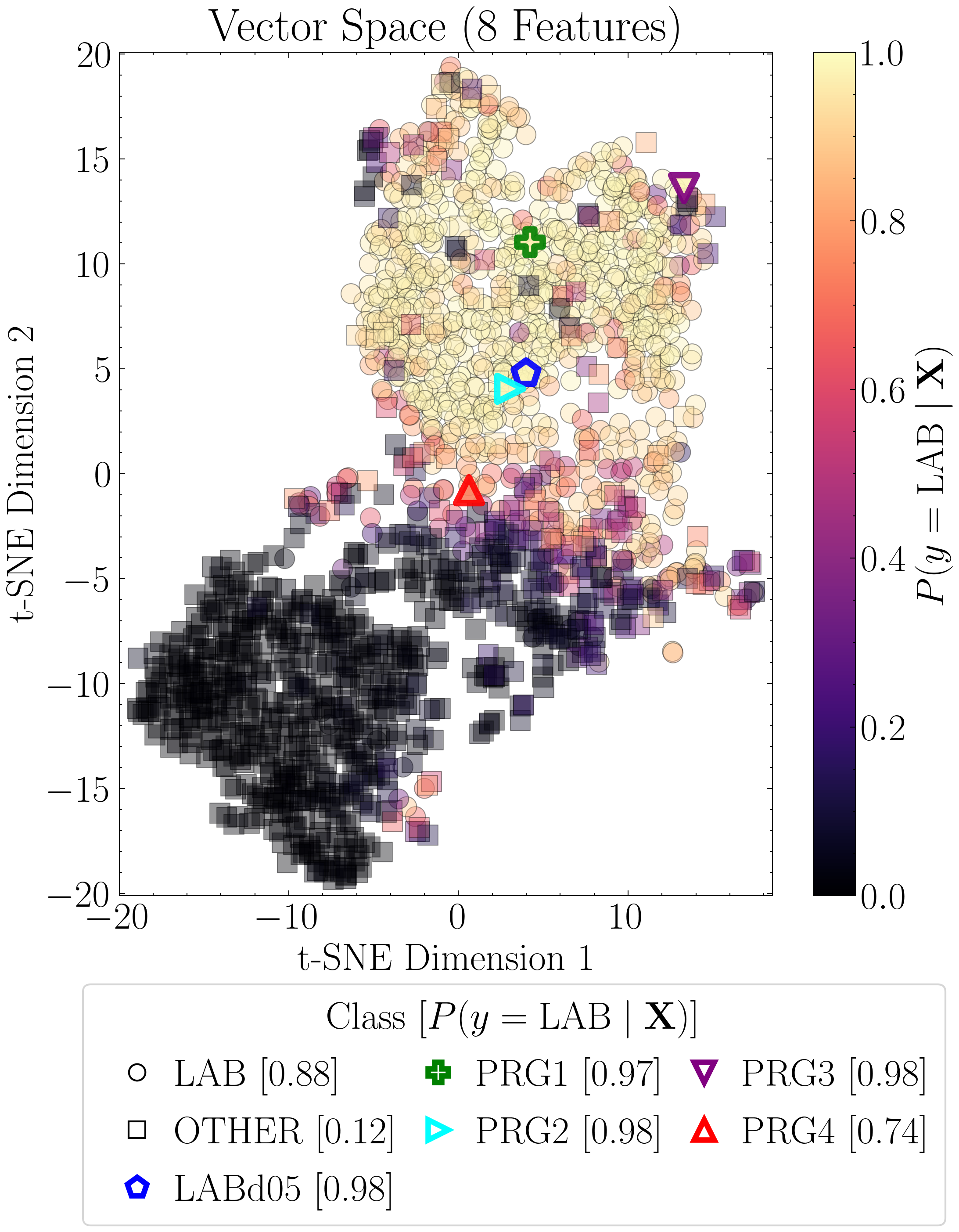
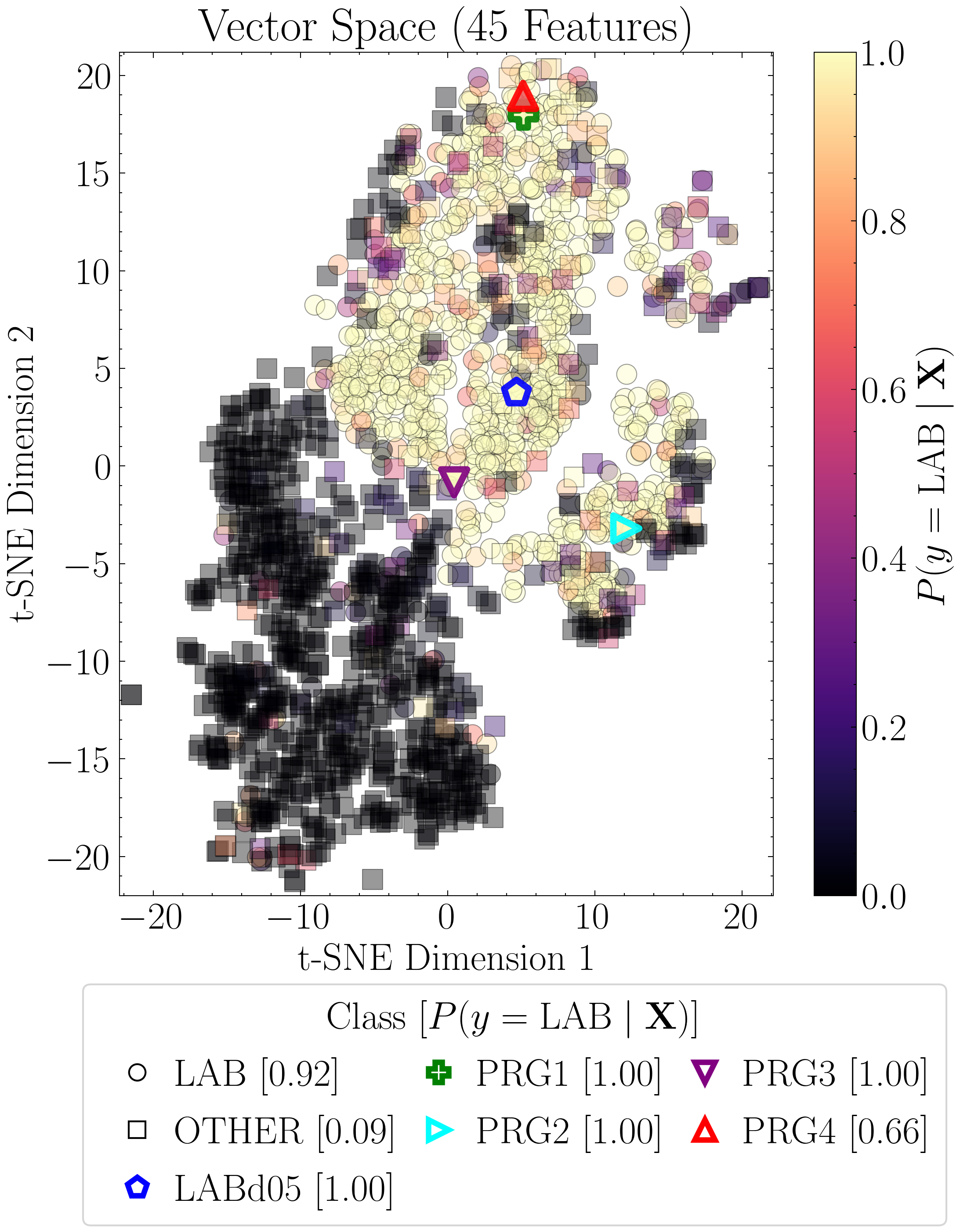
t-SNE Projections
With the LOO CV results, we can generate t-SNE projections and scale the points by their probability scores.
We first generate the t-SNE projections and save the scatter-point positions using the built-in methods of the Classifier class.
import numpy as np
import pandas as pd
from pyBIA import ensemble_model, data_processing

# Where the training set files were saved
nsig_path = 'nsigs/'

sig = 0.32 #The optimal sig threshold to apply as per Figure 2
df = pd.read_csv(f'{nsig_path}_Bw_training_set_nsig_{sig}')

# Log-transform the Hu moments
hu_cols = ['Hu1', 'Hu2', 'Hu3', 'Hu4', 'Hu5', 'Hu6', 'Hu7']
df[hu_cols] = df[hu_cols].apply(data_processing.signed_log_transform)

# Omit any non-detections
mask = np.where((df['area'] != -999) & np.isfinite(df['mag']) & np.all(np.isfinite(df[[f'Hu{i}' for i in range(1, 8)]]), axis=1))[0]

# Balance both classes to be of same size
blob_index = np.where(df['flag'].iloc[mask] == 1)[0]
other_index = np.where(df['flag'].iloc[mask] == 0)[0]
df_filtered = df.iloc[mask[np.concatenate((blob_index, other_index[:len(blob_index)]))]]

#These are the features to use, note that the catalog includes more than this!
columns = [
    'mag', 'mag_err',
    'M00', 'M10', 'M01', 'M20', 'M11', 'M02', 'M30', 'M21', 'M12', 'M03',
    'mu20', 'mu11', 'mu02', 'mu30', 'mu21', 'mu12', 'mu03',
    'G10', 'G01', 'G20', 'G11', 'G02', 'G30', 'G21', 'G12', 'G03',
    'Hu1', 'Hu2', 'Hu3', 'Hu4', 'Hu5', 'Hu6', 'Hu7',
    'L00', 'L10', 'L01', 'L20', 'L11', 'L02', 'L30', 'L21', 'L12', 'L03',
    'area', 'covar_sigx2', 'covar_sigy2', 'covar_sigxy', 'covariance_eigval1', 'covariance_eigval2',
    'cxx', 'cxy', 'cyy', 'eccentricity', 'ellipticity', 'elongation',
    'equivalent_radius', 'fwhm', 'gini', 'orientation', 'perimeter',
    'semimajor_sigma', 'semiminor_sigma', 'max_value', 'min_value'
]

# Training data arrays
data_x, data_y = np.array(df_filtered[columns]), np.array(df_filtered['flag'])
df_names = np.array(df_filtered.obj_name)

# Load the LoO Analysis results
loo_confirmed_lab = np.loadtxt('LoO_Confirmed_LAB', dtype=str)
loo_lab = np.loadtxt('LoO_LAB', dtype=str)
loo_other = np.loadtxt('LoO_OTHER', dtype=str)

#The names of our confirmed LABs as they appaer in the NDWFS Catalog: 'LABd05', 'PRG1', 'PRG2', 'PRG3', 'PRG4'
confirmed_LAB_cat_names = ['NDWFS_J143410.9+331730','NDWFS_J143512.2+351108','NDWFS_J142623.0+351422','NDWFS_J143412.7+332939', 'NDWFS_J142653.1+343856']

# Concat the data from all three models (base, xgboost-8, xgboost-45)
# The first column contains the na,es the second the baseline model data, 3rd column is xgboost-8, fourth is xgboost-45
names = np.r_[loo_lab[:,0], confirmed_LAB_cat_names, loo_other[:,0]]
probas_xgboost_8 = np.r_[loo_lab[:,2], loo_confirmed_lab[:,2], loo_other[:,2]]
probas_xgboost_45 = np.r_[loo_lab[:,3], loo_confirmed_lab[:,3], loo_other[:,3]]

# Sort in order of the training data (df_filtered)
indices = []
for i in range(len(df_names)):
    indices.append(np.where(names == df_names[i])[0][0])

names = names[indices]
probas_xgboost_8, probas_xgboost_45 = probas_xgboost_8[indices].astype('float'), probas_xgboost_45[indices].astype('float')

# Load the models (saved in earlier code)
clf = 'xgb' # The classification model
impute = False # Will not impute NaN values, as they should not be present after masking non-detections
xgboost_8_model = ensemble_model.Classifier(data_x, data_y, clf=clf, impute=impute)
xgboost_8_model.load('ensemble_model_xgb_boruta_xgb')

xgboost_45_model = ensemble_model.Classifier(data_x, data_y, clf=clf, impute=impute)
xgboost_45_model.load('ensemble_model_xgb_boruta_rf')

# For plotting purposes change the labels from numeric to text
y_labels = ['LAB' if flag == 1 else 'OTHER' for flag in data_y]

# For plotting purposes, re-name the five confirmed blobs to Confirmed LyAlpha
confirmed_names = np.loadtxt('confirmed_LAB_names.txt', dtype=str)

# Identify the confirmed LABs and re-name
for name in confirmed_names:
    index = np.where(df_filtered.obj_name == name)[0][0]
    y_labels[index] = r'Confirmed_Ly$\alpha$'

# The t-SNE projection with custom y_data labels, highlighting the scatter points for the confirmed blobs
# For now we only need to generate the t-SNE projection and save the scatter point positions
return_data = True # Whether to also return the x and y coordinates of the scatter points (will correspond to the order of the feature matrix (i.e., your labels in `data_y`))

x_8, y_8 = xgboost_8_model.plot_tsne(data_y=y_labels, return_data=return_data)
x_45, y_45 = xgboost_45_model.plot_tsne(data_y=y_labels, return_data=return_data)

np.savetxt('tsne_scatter_data_8_feats.txt', np.c_[x_8, y_8, y_labels, names, probas_xgboost_8],fmt='%s',header='x, y, labels, names, probas')
np.savetxt('tsne_scatter_data_45_feats.txt', np.c_[x_45, y_45, y_labels, names, probas_xgboost_45],fmt='%s',header='x, y, labels, names, probas')
The t-SNE projection data files are available for download:
We can now plot the t-SNE projections, with point sizes scaled by their predicted probabilities.
import numpy as np
import matplotlib.pyplot as plt
import matplotlib as mpl
import scienceplots
plt.style.use('science')
plt.rcParams.update({'font.size': 21})

# Loop runs twice, once with model='xgboost_8' and the other with model='xgboost_45'
for model in ['xgboost_8', 'xgboost_45']:

        fname = 'tsne_scatter_data_8_feats.txt' if model == 'xgboost_8' else 'tsne_scatter_data_45_feats.txt'

        # Load the t-SNE data saved in code above
        xgb_results = np.loadtxt(fname, dtype=str)
        x, y = xgb_results[:, 0].astype(float), xgb_results[:, 1].astype(float)
        labels = xgb_results[:, 2]
        names = xgb_results[:, 3]
        probas = xgb_results[:, 4].astype(float)

        marker_dict = {'LAB': 'o', 'OTHER': 's'}
        cmap, norm = plt.get_cmap('magma'), mpl.colors.Normalize(0, 1)

        # To track the confirmed LABs
        special_objects = {
            'NDWFS_J143410.9+331730': 'LABd05',
            'NDWFS_J143512.2+351108': 'PRG1',
            'NDWFS_J142623.0+351422': 'PRG2',
            'NDWFS_J143412.7+332939': 'PRG3',
            'NDWFS_J142653.1+343856': 'PRG4'
        }

        special_colors  = ['blue', 'green', 'cyan', 'purple', 'red']
        special_markers = ['p', 'P', '>', 'v', '^']

        # PLOT
        legend_space = 5.3
        fig, ax = plt.subplots(figsize=(8, 8 + legend_space))
        fig.subplots_adjust(bottom=legend_space / (8 + legend_space))

        # Don't plot the confirmed LABs these are done separately
        for cls in np.unique(labels):
            # Skip the confirmed LABs
            if cls == 'Confirmed_Ly$\\alpha$':
                continue

            mask = labels == cls
            ax.scatter(x[mask], y[mask], c=probas[mask], cmap=cmap, norm=norm, marker=marker_dict[cls], s=120, edgecolor='black', linewidth=.5, alpha=.4)

        # Now include the confirmed LABs
        for i, (name, short) in enumerate(special_objects.items()):
            mask = names == name
            ax.scatter(x[mask], y[mask], c=probas[mask], cmap=cmap, norm=norm, marker=special_markers[i], s=200, edgecolor=special_colors[i], linewidth=3.5, alpha=.9)

        sm = mpl.cm.ScalarMappable(norm=norm, cmap=cmap)
        sm.set_array([])
        cbar = fig.colorbar(sm, ax=ax)#, extend='none')
        cbar.set_label(r"$P(y=\mathrm{LAB}\mid\mathbf{X})$")

        handles = [
            mpl.lines.Line2D([], [], marker='o', mfc='none', mec='black', markersize=9, linestyle='None', label=f"LAB [{probas[labels=='LAB'].mean():.2f}]"),
            mpl.lines.Line2D([], [], marker='s', mfc='none', mec='black', markersize=9, linestyle='None', label=f"OTHER [{probas[labels=='OTHER'].mean():.2f}]")
        ]

        for i, (name, short) in enumerate(special_objects.items()):
            p = probas[names == name][0]
            handles.append(mpl.lines.Line2D([], [], marker=special_markers[i], mfc='none', mec=special_colors[i], markeredgewidth=3., markersize=11, linestyle='None', label=f"{short} [{p:.2f}]"))

        fig.legend(handles=handles, loc='lower center', bbox_to_anchor=(0.5, legend_space / 2 / (8 + legend_space)), ncol=3, frameon=True, fancybox=True, columnspacing=0.05, handletextpad=0, title=r'Class [$P(y=\mathrm{LAB}\mid\mathbf{X})$]')

        if model == 'xgboost_8':
            ax.set_xlim(-20, 18.5); ax.set_ylim(-20.1, 20.1)
        else:
            ax.set_xlim(-22.3, 22.1); ax.set_ylim(-22., 21.2)

        ax.set_title("Vector Space (8 Features)" if model == 'xgboost_8' else "Vector Space (45 Features)")
        ax.set_xlabel("t-SNE Dimension 1")
        ax.set_ylabel("t-SNE Dimension 2")

        plt.savefig(f'tsne_new_{"45" if model == 'xgboost_45' else "8"}.png', dpi=300, bbox_inches='tight')
        plt.show()
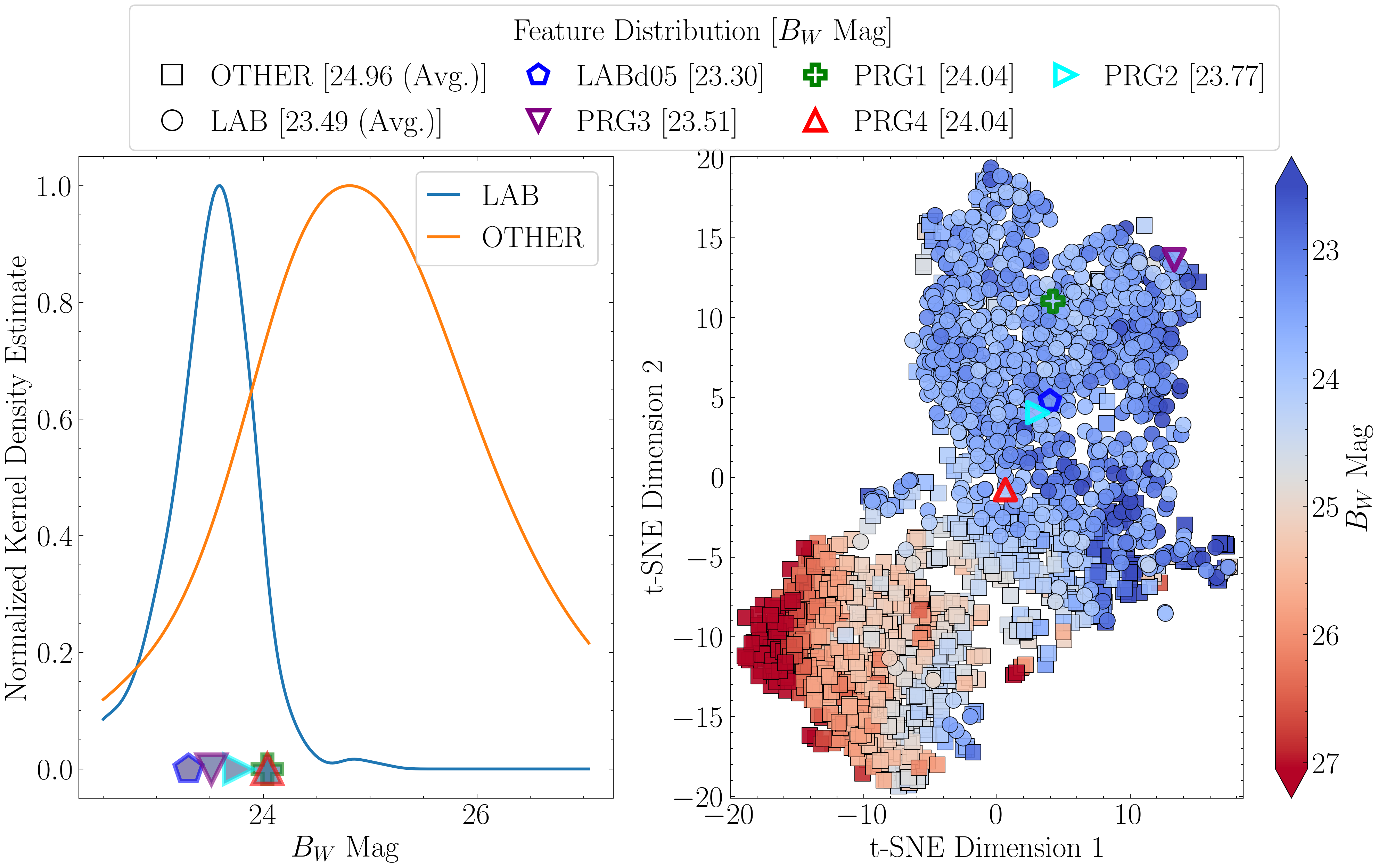
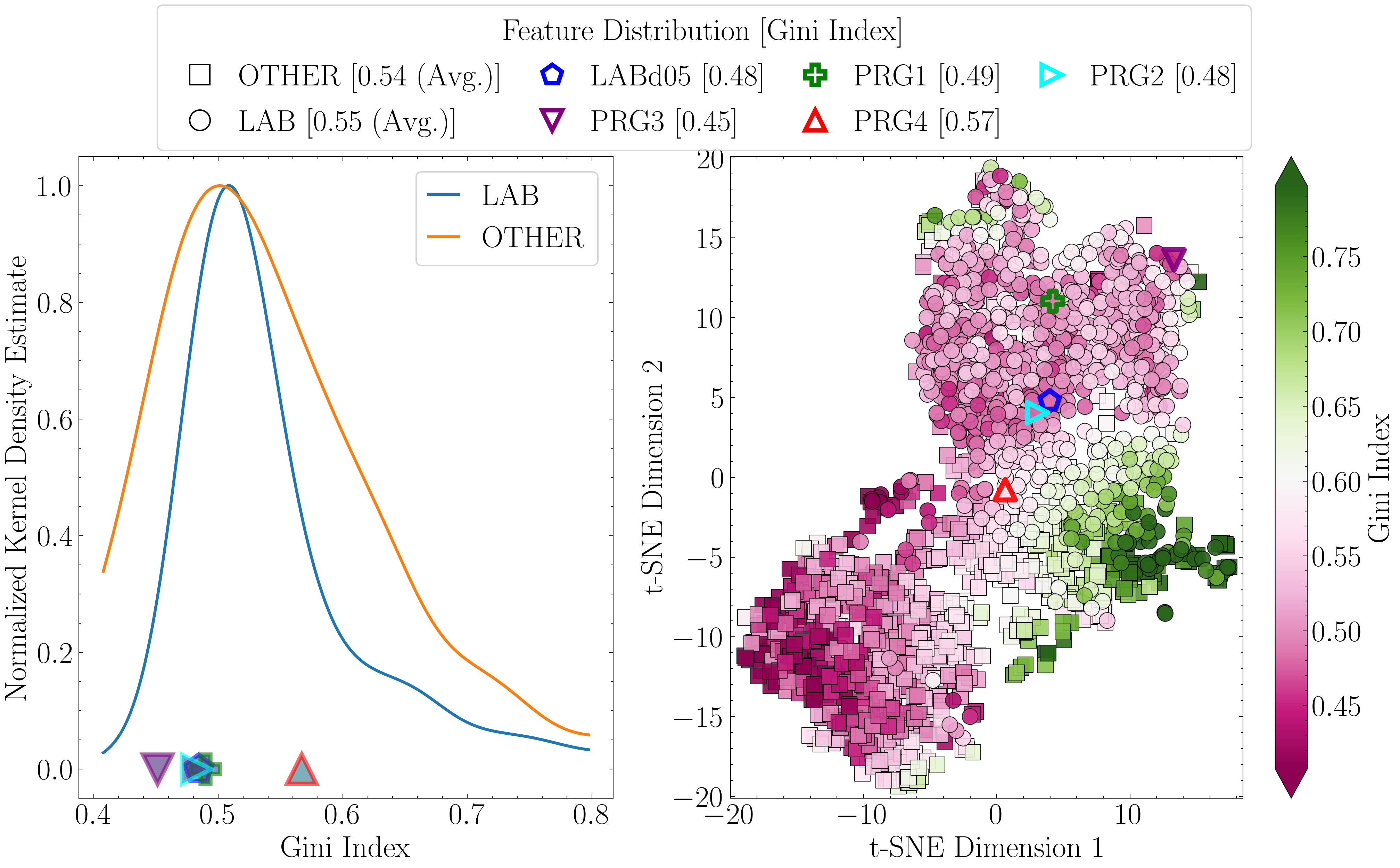
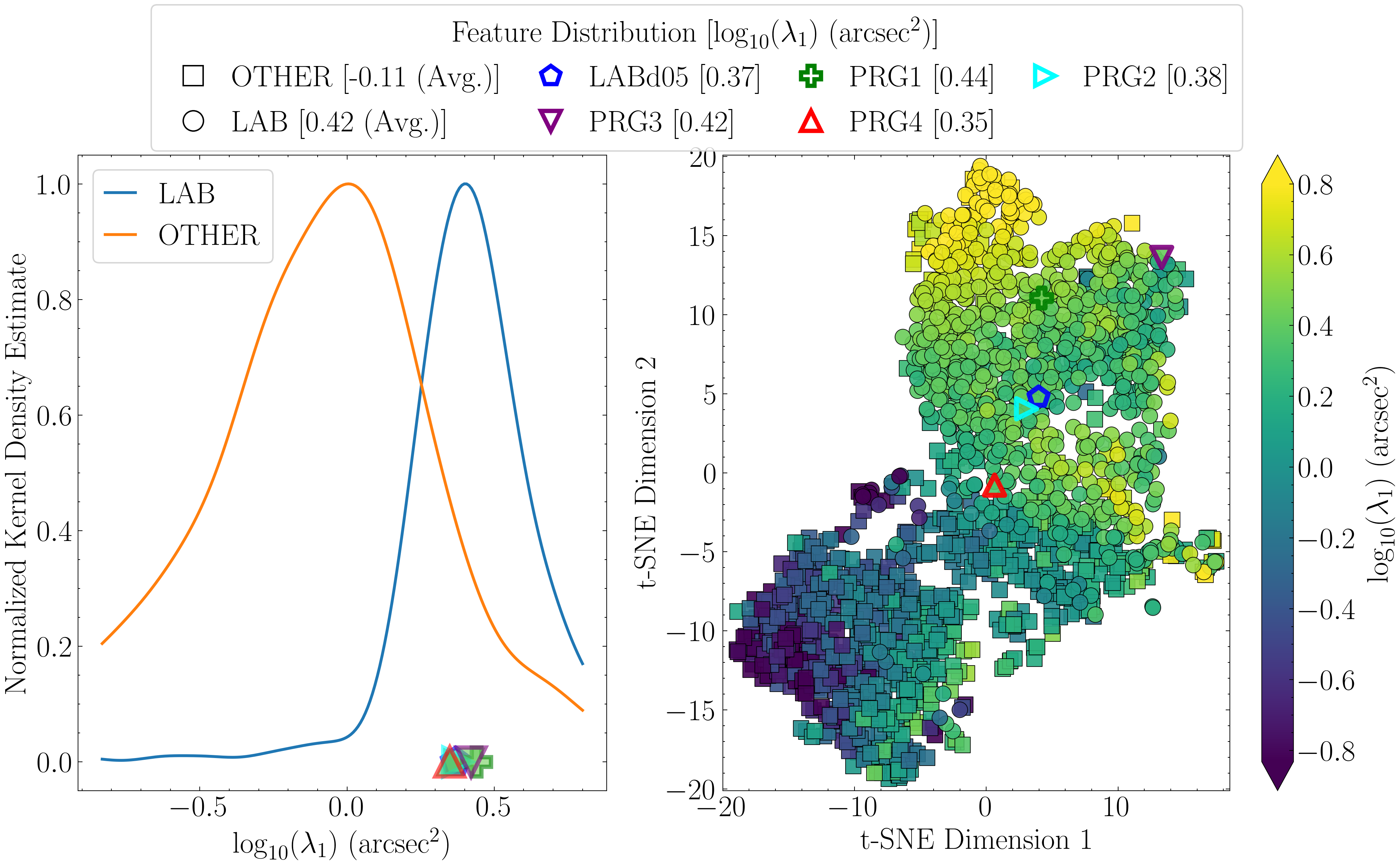
Next, we re-compute the t-SNE projections, this time scaling the points by the values of the top three features. Each projection is paired with a Gaussian kernel density estimate (KDE) of that feature for LAB and OTHER, normalized to unit height, to summarize the class-wise distributions.
import re
import numpy as np
import pandas as pd
from scipy.stats import gaussian_kde
import matplotlib as mpl
from matplotlib.lines import Line2D
import matplotlib.pyplot as plt
import scienceplots
plt.style.use('science')
plt.rcParams.update({'font.size': 21})

# Where the training set files were saved
nsig_path = 'nsigs/'

# Load training data
sig = 0.32
df = pd.read_csv(f'{nsig_path}_Bw_training_set_nsig_{sig}')
mask = np.where((df['area'] != -999) & np.isfinite(df['mag']) & np.isfinite(df['mag_err']))[0]
blob_index = np.where(df['flag'].iloc[mask] == 1)[0]
other_index = np.where(df['flag'].iloc[mask] == 0)[0]
df_filtered = df.iloc[mask[np.concatenate((blob_index, other_index[:len(blob_index)]))]]

# Load t-SNE projection data
xgb_results = np.loadtxt('tsne_scatter_data_8_feats.txt', dtype=str)
x = xgb_results[:, 0].astype(float)
y = xgb_results[:, 1].astype(float)
y_labels = xgb_results[:, 2]

# For the labels
special_objects = {
    'NDWFS_J143410.9+331730': 'LABd05',
    'NDWFS_J143512.2+351108': 'PRG1',
    'NDWFS_J142623.0+351422': 'PRG2',
    'NDWFS_J143412.7+332939': 'PRG3',
    'NDWFS_J142653.1+343856': 'PRG4'
}
special_colors = ['blue', 'green', 'cyan', 'purple', 'red']
special_markers = ['p', 'P', '>', 'v', '^']

# Top features to show
important_cols = ['mag', 'gini', 'covariance_eigval1']
titles = [r'$B_W$ Mag', 'Gini Index', r'$\rm \log_{10}$($\lambda_1$) ($\rm arcsec^2$)']

# Pix to arcsec conversion factor for NDWFS Bootes
pix_conversion = 3.8961
pix_to_arcsec2 = pix_conversion ** 2

def process_feature_array(values, col):
    # To log-scale and convert to physical units
    v = values.astype(float)
    if col == 'covariance_eigval1':
        v = v / pix_to_arcsec2
        v = np.log10(v)
    return v

def process_single_value(val, col):
    # To log-scale and convert to physical units (for confirmed LABs only)
    t = float(val)
    if col == 'covariance_eigval1':
        t = t / pix_to_arcsec2
        t = np.log10(t)
    return t

# Loop and plot each one separately
for col_, title_ in zip(important_cols, titles):

    if col_ == 'mag':
        cmap_to_use = 'coolwarm'
    elif col_ == 'gini':
        cmap_to_use = 'PiYG'
    else:
        cmap_to_use = 'viridis'

    raw_feature_vals = np.array(df_filtered[col_])
    feature_vals = process_feature_array(raw_feature_vals, col_)

    lo, hi = np.percentile(feature_vals, [3, 97])
    norm = mpl.colors.Normalize(vmin=lo, vmax=hi, clip=True)

    marker_dict = {'Confirmed_Ly$\\alpha$': '*', 'LAB': 'o', 'OTHER': 's'}
    label_dict = {'LAB': 'LAB', 'OTHER': 'OTHER'}

    fig, (ax_kde, ax_tsne) = plt.subplots(ncols=2, figsize=(16, 8), gridspec_kw={'width_ratios': [1, 1.2]})

    lab_mask = (y_labels == 'Confirmed_Ly$\\alpha$') | (y_labels == 'LAB')
    other_mask = (y_labels == 'OTHER')

    x_grid = np.linspace(lo, hi, 200)
    density_lab = np.zeros_like(x_grid)
    density_other = np.zeros_like(x_grid)

    if np.sum(lab_mask) > 1:
        dl = gaussian_kde(feature_vals[lab_mask])(x_grid)
        if dl.max() > 0: density_lab = dl / dl.max()
    if np.sum(other_mask) > 1:
        do = gaussian_kde(feature_vals[other_mask])(x_grid)
        if do.max() > 0: density_other = do / do.max()

    ax_kde.plot(x_grid, density_lab, label='LAB', color='tab:blue', lw=2)
    ax_kde.plot(x_grid, density_other, label='OTHER', color='tab:orange', lw=2)
    ax_kde.set_xlabel(title_)
    ax_kde.set_ylabel('Normalized Kernel Density Estimate')
    ax_kde.legend(loc=('upper left' if col_ == 'covariance_eigval1' else 'upper right'), frameon=True, fancybox=True, handlelength=1)

    for i, (obj_name, label_obj) in enumerate(special_objects.items()):
        arr = df_filtered.loc[df_filtered['obj_name'] == obj_name, col_].values
        if arr.size > 0:
            sval = process_single_value(arr[0], col_)
            color_special = mpl.cm.viridis(norm(sval))
            ax_kde.plot(sval, 0, marker=special_markers[i], markersize=20,
                        markerfacecolor=color_special, markeredgecolor=special_colors[i],
                        linewidth=3.5, markeredgewidth=3., alpha=0.6)

    cmap = plt.get_cmap(cmap_to_use)
    for cls in np.unique(y_labels)[::-1]:

        if cls == 'Confirmed_Ly$\\alpha$':
            continue

        cls_mask = (y_labels == cls)
        ax_tsne.scatter(
            x[cls_mask], y[cls_mask],
            c=feature_vals[cls_mask],
            cmap=cmap, norm=norm,
            marker=marker_dict.get(cls, 'o'),
            s=120, edgecolor='black', linewidth=0.5, alpha=0.9
        )

    for i, (obj_name, label_obj) in enumerate(special_objects.items()):
        tsne_mask = (np.array(xgb_results[:, 3]) == obj_name)
        if tsne_mask.any():
            ax_tsne.scatter(
                x[tsne_mask], y[tsne_mask],
                c=feature_vals[tsne_mask],
                cmap=cmap, norm=norm,
                marker=special_markers[i],
                s=200, edgecolor=special_colors[i],
                linewidth=3.5, alpha=0.9
            )

    sm = mpl.cm.ScalarMappable(norm=norm, cmap=cmap)
    sm.set_array([])
    cbar = fig.colorbar(sm, ax=ax_tsne, extend='both')

    if col_ == 'mag':
        cbar.ax.invert_yaxis()

    cbar.set_label(title_)

    ax_tsne.set_xlabel("t-SNE Dimension 1")
    ax_tsne.set_ylabel("t-SNE Dimension 2")
    ax_tsne.set_xlim(-20, 18.5)
    ax_tsne.set_ylim(-20.1, 20.1)

    tsne_handles, tsne_labels = [], []
    for cls in np.unique(y_labels)[::-1]:

        if cls == 'Confirmed_Ly$\\alpha$':
            continue

        cls_mask = (y_labels == cls)
        mean_val = np.mean(feature_vals[cls_mask]) if np.any(cls_mask) else np.nan
        m = marker_dict.get(cls, 'o')
        line = Line2D([], [], marker=m, color='black', markerfacecolor='none', linestyle='None', linewidth=1, markersize=np.sqrt(200))
        tsne_handles.append(line)
        tsne_labels.append(f"{label_dict.get(cls, cls)} [{mean_val:.2f} (Avg.)]")

    for i, (obj_name, label_obj) in enumerate(special_objects.items()):
        tsne_mask = (np.array(xgb_results[:, 3]) == obj_name)
        if tsne_mask.any():
            val_for_obj = feature_vals[tsne_mask][0]
            line = Line2D([], [], marker=special_markers[i], color=special_colors[i],
                          markerfacecolor='none', markeredgewidth=3., linestyle='None',
                          linewidth=1., markersize=np.sqrt(200))
            tsne_handles.append(line)
            tsne_labels.append(f"{label_obj} [{val_for_obj:.2f}]")

    ncols = 4
    row1_desired = ['OTHER', 'LABd05', 'PRG1', 'PRG2']
    row2_desired = ['LAB', 'PRG3', 'PRG4']

    def _base_name(lbl): return re.split(r'\s*\[', lbl)[0].strip()

    name_to_idx = {}
    for i, lbl in enumerate(tsne_labels):
        nm = _base_name(lbl)
        if nm not in name_to_idx:
            name_to_idx[nm] = i

    order_names, used = [], set()
    for j in range(ncols):
        if j < len(row1_desired): order_names.append(row1_desired[j])
        if j < len(row2_desired): order_names.append(row2_desired[j])

    ordered_handles, ordered_labels = [], []
    for nm in order_names:
        if nm in name_to_idx and nm not in used:
            k = name_to_idx[nm]
            ordered_handles.append(tsne_handles[k])
            ordered_labels.append(tsne_labels[k])
            used.add(nm)

    fig.legend(handles=ordered_handles, labels=ordered_labels,
               loc='upper center', ncol=ncols, frameon=True, fancybox=True,
               columnspacing=0.6, handletextpad=0.3,
               title=fr'Feature Distribution [{title_}]',
               bbox_to_anchor=(0.5, 1.08))

    plt.savefig(f'kde_tsne_new_8_{col_}.png', dpi=300, bbox_inches='tight')
    plt.show()
    plt.clf()
    plt.close()
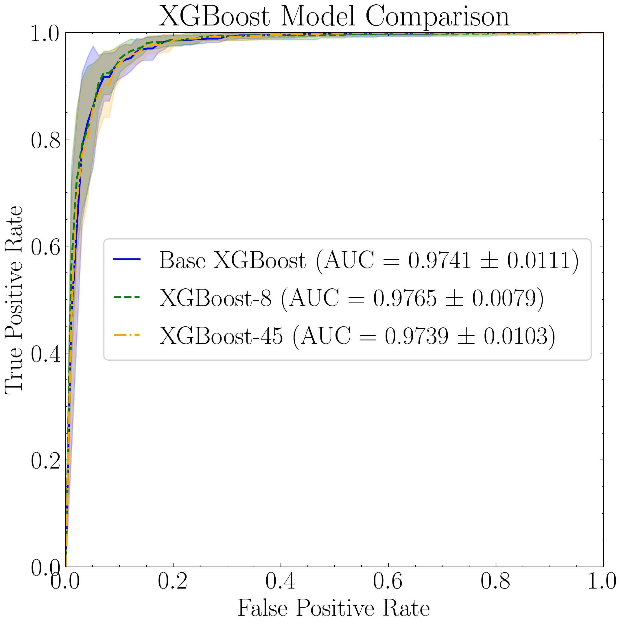
XGBoost Model Performance
We now assess the performance of the three XGBoost models, beginning with a ROC curve evaluated using 10-fold cross-validation.
import numpy as np
import pandas as pd
from sklearn.model_selection import StratifiedKFold
from sklearn.metrics import roc_curve, auc
from pyBIA import ensemble_model, data_processing
import matplotlib.pyplot as plt
import scienceplots
plt.style.use('science')
plt.rcParams.update({'font.size': 21})

# Where the training set files were saved
nsig_path = 'nsigs/'

sig = 0.32 #The optimal sig threshold to apply as per Figure 2
df = pd.read_csv(f'{nsig_path}_Bw_training_set_nsig_{sig}')
hu_cols = ['Hu1', 'Hu2', 'Hu3', 'Hu4', 'Hu5', 'Hu6', 'Hu7']
df[hu_cols] = df[hu_cols].apply(data_processing.signed_log_transform)

# Omit any non-detections
mask = np.where((df['area'] != -999) & np.isfinite(df['mag']) & np.all(np.isfinite(df[[f'Hu{i}' for i in range(1, 8)]]), axis=1))[0]

# Balance both classes to be of same size
blob_index = np.where(df['flag'].iloc[mask] == 1)[0]
other_index = np.where(df['flag'].iloc[mask] == 0)[0]
df_filtered = df.iloc[mask[np.concatenate((blob_index, other_index[:len(blob_index)]))]]

#These are the features to use, note that the catalog includes more than this!
columns = [
    'mag', 'mag_err',
    'M00', 'M10', 'M01', 'M20', 'M11', 'M02', 'M30', 'M21', 'M12', 'M03',
    'mu20', 'mu11', 'mu02', 'mu30', 'mu21', 'mu12', 'mu03',
    'G10', 'G01', 'G20', 'G11', 'G02', 'G30', 'G21', 'G12', 'G03',
    'Hu1', 'Hu2', 'Hu3', 'Hu4', 'Hu5', 'Hu6', 'Hu7',
    'L00', 'L10', 'L01', 'L20', 'L11', 'L02', 'L30', 'L21', 'L12', 'L03',
    'area', 'covar_sigx2', 'covar_sigy2', 'covar_sigxy', 'covariance_eigval1', 'covariance_eigval2',
    'cxx', 'cxy', 'cyy', 'eccentricity', 'ellipticity', 'elongation',
    'equivalent_radius', 'fwhm', 'gini', 'orientation', 'perimeter',
    'semimajor_sigma', 'semiminor_sigma', 'max_value', 'min_value'
]

df_names = np.array(df_filtered.obj_name)

# Training data arrays
data_x, data_y = np.array(df_filtered[columns]), np.array(df_filtered['flag'])

# This is the base model, no hyperparameter optimization, uses all the features
clf = 'xgb' # The classification model that will be trined
impute = False # Whether to impute missing values (NaN)
base_model = ensemble_model.Classifier(data_x, data_y, clf=clf, impute=impute)
base_model.create()
BASE_M = base_model.model

# This is the optimized model trained with 8 features
xgboost_8_model = ensemble_model.Classifier(data_x, data_y, clf=clf, impute=impute)
xgboost_8_model.load('ensemble_model_xgb_boruta_xgb')
OPT_M1 = xgboost_8_model.model

# This is the optimized model trained with 45 features
xgboost_45_model = ensemble_model.Classifier(data_x, data_y, clf=clf, impute=impute)
xgboost_45_model.load('ensemble_model_xgb_boruta_rf')
OPT_M2 = xgboost_45_model.model

# Plot ROC Curves with 10-fold cross-validation

# Define a dictionary mapping model names to model objects.
models = {
    "Base XGBoost": BASE_M,
    "XGBoost-8": OPT_M1,
    "XGBoost-45": OPT_M2,
}

# Choose different colors and line styles for each model.
model_colors = {
    "Base XGBoost": "blue",
    "XGBoost-8": "green",
    "XGBoost-45": "orange",
}

model_linestyles = {
    "Base XGBoost": "-",
    "XGBoost-8": "--",
    "XGBoost-45": "-.",
}

# Set up 10-fold cross-validation
opt_cv = 10 # Will perform 10-fold cross validation
SEED_NO = 1909 # Random seed for the CV

cv = StratifiedKFold(n_splits=opt_cv, shuffle=True, random_state=SEED_NO)

# Define a common grid of false positive rates at which we will interpolate the TPR
mean_fpr = np.linspace(0, 1, 100)

plt.figure(figsize=(8, 8))

# Loop over the three models.
for model_name, model in models.items():

    # To store TPR and corresponding AUC
    tprs, aucs = [], []

    # Loop over the CV folds.
    for train_idx, test_idx in cv.split(data_x, data_y):

        # Fit the model on the training fold
        model.fit(data_x[train_idx], data_y[train_idx])

        # Get the predicted probabilities for the positive class on the test fold
        y_proba = model.predict_proba(data_x[test_idx])[:, 1]

        # Compute the ROC curve and AUC for this fold
        fpr, tpr, _ = roc_curve(data_y[test_idx], y_proba)
        fold_auc = auc(fpr, tpr)
        aucs.append(fold_auc)

        # Interpolate the TPR at the mean_fpr points
        interp_tpr = np.interp(mean_fpr, fpr, tpr)
        interp_tpr[0] = 0.0 # Ensure the curve starts at 0
        tprs.append(interp_tpr)

    # Compute the mean and std TPR values across folds.
    mean_tpr = np.mean(tprs, axis=0)
    mean_tpr[-1] = 1.0 # To ensure the curve ends at 1
    std_tpr = np.std(tprs, axis=0)

    # Compute the mean and std AUC.
    mean_auc = np.mean(aucs) # average of the per‑fold AUCs
    std_auc = np.std(aucs)

    # Plot the mean ROC curve for this model.
    plt.plot(
        mean_fpr,
        mean_tpr,
        color=model_colors[model_name],
        linestyle=model_linestyles[model_name],
        lw=1.6,
        label=fr"{model_name} (AUC = {mean_auc:0.4f} $\pm$ {std_auc:0.4f})"
    )

    # Plot the standard deviation shaded region
    tpr_upper = np.minimum(mean_tpr + std_tpr, 1)
    tpr_lower = np.maximum(mean_tpr - std_tpr, 0)
    plt.fill_between(mean_fpr, tpr_lower, tpr_upper, color=model_colors[model_name], alpha=0.2)

plt.xlim([0, 1]); plt.ylim([0, 1])
plt.xlabel("False Positive Rate")
plt.ylabel("True Positive Rate")
plt.title("XGBoost Model Comparison")
plt.legend(loc="center right", handlelength=1, frameon=True, fancybox=True)
plt.savefig('new_rocs.png', dpi=300, bbox_inches='tight')
plt.show()
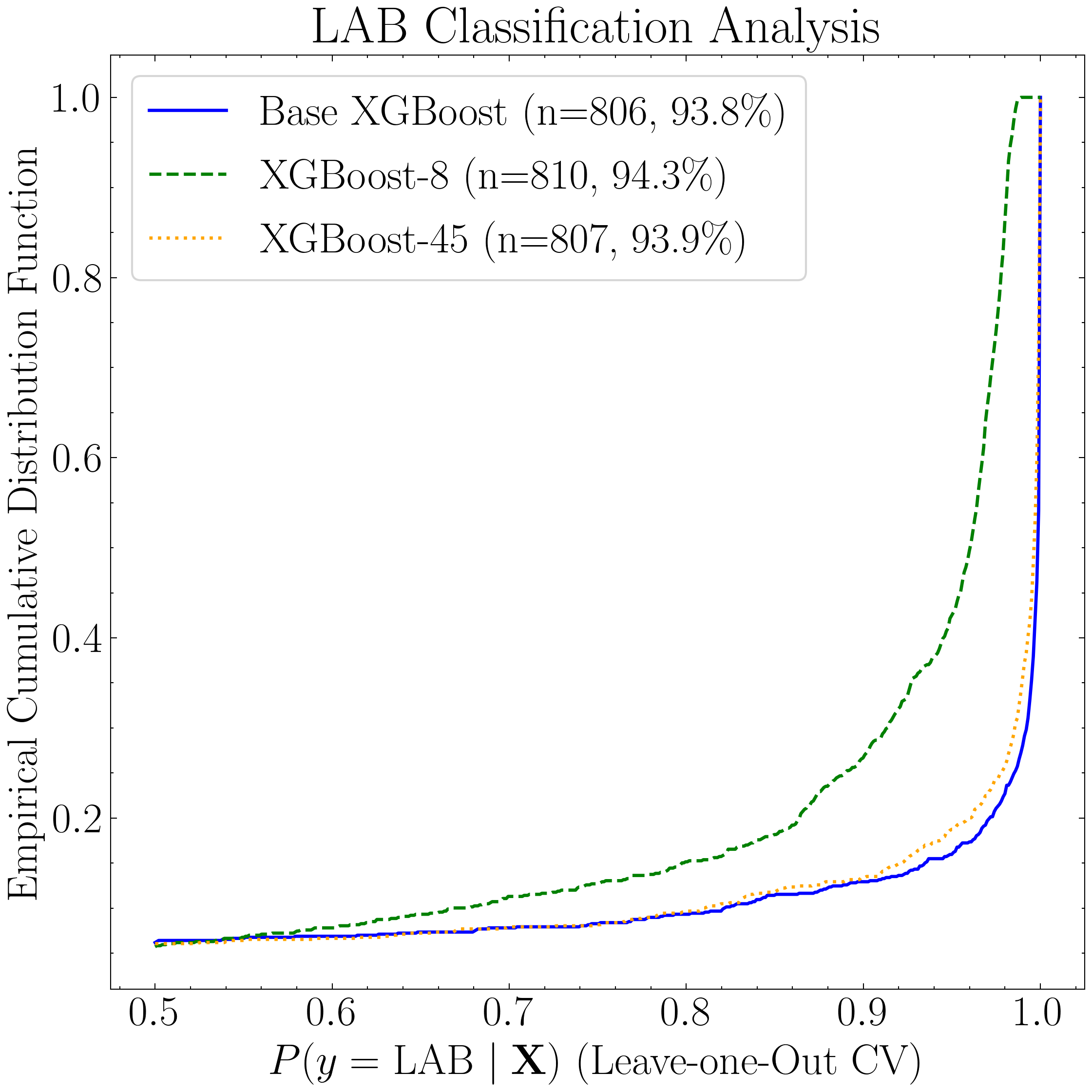
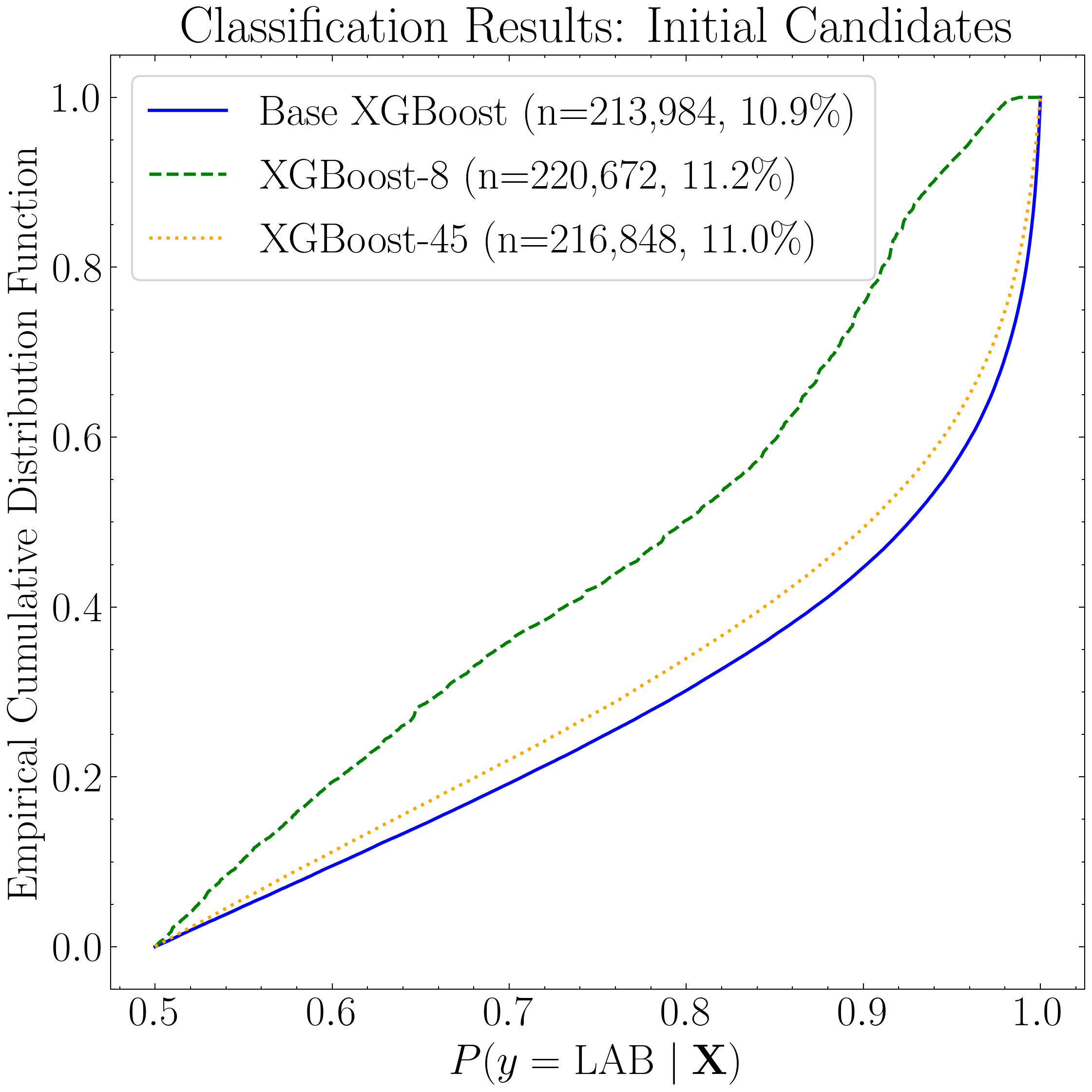
Next, we generate empirical cumulative distribution functions (eCDFs) to evaluate how many positive detections each model produces as a function of predicted probability—both for the candidate catalogs (the positively classified objects in the NDWFS Boötes field saved earlier) and for the LAB training instances that were also positively classified as per the LOO CV.
import numpy as np
import pandas as pd
from pyBIA import data_processing
import matplotlib.pyplot as plt
import scienceplots
plt.style.use("science")
plt.rcParams.update({"font.size": 21})

# First load the master catalog and count how many objects there are (for normalization)
other_all = pd.read_csv('Other_Catalog_Master_0.32')

# Omit non-detections and record total number of detections
mask = np.where((other_all['area'] != -999) & np.isfinite(other_all['mag']) & np.all(np.isfinite(other_all[[f'Hu{i}' for i in range(1, 8)]]), axis=1))[0]
total_no = len(mask)

def ecdf_common(data, x_grid):
    """Compute the eCDF evaluated on a common grid."""
    sorted_data = np.sort(data)
    # For each value in the common grid, count the fraction of data points <= x.
    counts = np.searchsorted(sorted_data, x_grid, side='right')
    return counts / len(sorted_data)

# Load the candidate catalogs and LOO analysis results saved before

# Model 1: Baseline XGBoost
# Candidate probabilities
df_model1 = pd.read_csv('candidate_catalog_base.csv')
probas_cand_m1 = np.array(df_model1.proba)

# Load results from Leave-one-Out analysis
LoO_LAB = np.loadtxt('LoO_LAB', dtype=str)
LoO_Confirmed_LAB = np.loadtxt('LoO_Confirmed_LAB', dtype=str)

# For Baseline XGBoost, probas saved in second column
train_m1 = np.r_[LoO_LAB[:, 1].astype(float), LoO_Confirmed_LAB[:, 1].astype(float)]

# Model 2: XGBoost-8
# Candidate probabilities
df_model2 = pd.read_csv('candidate_catalog_optimized_xgboost_8.csv')
probas_cand_m2 = np.array(df_model2.proba)

# For XGBoost-8, probas saved in third column
train_m2 = np.r_[LoO_LAB[:, 2].astype(float), LoO_Confirmed_LAB[:, 2].astype(float)]

# Model 3: XGBoost-45
# Candidate probabilities
df_model3 = pd.read_csv('candidate_catalog_optimized_xgboost_45.csv')
probas_cand_m3 = np.array(df_model3.proba)

# For XGBoost-45, probas saved in third column
train_m3 = np.r_[LoO_LAB[:, 3].astype(float), LoO_Confirmed_LAB[:, 3].astype(float)]

# Define a common x-grid (from 0.5 to 1.0) for all eCDF curves.
common_x = np.linspace(0.5, 1.0, 500)

# Compute eCDF for Candidates
ecdf_m1_cand = ecdf_common(probas_cand_m1, common_x)
ecdf_m2_cand = ecdf_common(probas_cand_m2, common_x)
ecdf_m3_cand = ecdf_common(probas_cand_m3, common_x)

# Compute eCDF for LAB training samples (which already include confirmed values)
ecdf_m1_lab = ecdf_common(train_m1, common_x)
ecdf_m2_lab = ecdf_common(train_m2, common_x)
ecdf_m3_lab = ecdf_common(train_m3, common_x)

# Set a common color for the curves
common_color =  ['blue', 'green', 'orange']

# Plot the Candidates eCDF
fig1, ax1 = plt.subplots(figsize=(8, 8))

# Plot using different line styles for clarity.
ax1.plot(common_x, ecdf_m1_cand, linestyle='-',  color=common_color[0], lw=1.6,
         label=f'Base XGBoost (n={len(probas_cand_m1):,}, {np.round(100*len(probas_cand_m1)/total_no,1)}\\%)')
ax1.plot(common_x, ecdf_m2_cand, linestyle='--', color=common_color[1], lw=1.6,
         label=f'XGBoost-8 (n={len(probas_cand_m2):,}, {np.round(100*len(probas_cand_m2)/total_no,1)}\\%)')
ax1.plot(common_x, ecdf_m3_cand, linestyle=':',  color=common_color[2], lw=1.6,
         label=f'XGBoost-45 (n={len(probas_cand_m3):,}, {np.round(100*len(probas_cand_m3)/total_no,1)}\\%)')

ax1.set_xlabel(r"$P(y =$ LAB $\mid \mathbf{{X}})$")
ax1.set_ylabel('Empirical Cumulative Distribution Function')# (ECDFs)')
ax1.set_title('Classification Results: Initial Candidates')
ax1.legend(loc='upper left', frameon=True, fancybox=True, handlelength=1.8)
plt.tight_layout()
plt.savefig('Candidates_eCDF.png', bbox_inches='tight', dpi=300)
plt.show()

# Plot the LAB eCDF
fig2, ax2 = plt.subplots(figsize=(8, 8))

# Plot the LAB eCDF curves for the three models.
ax2.plot(common_x, ecdf_m1_lab, linestyle='-',  color=common_color[0], lw=1.6,
         label=f'Base XGBoost (n={len(np.where(train_m1>=0.5)[0])}, {np.round(100*len(np.where(train_m1>=0.5)[0])/859,1)}\\%)')
ax2.plot(common_x, ecdf_m2_lab, linestyle='--', color=common_color[1], lw=1.6,
         label=f'XGBoost-8 (n={len(np.where(train_m2>=0.5)[0])}, {np.round(100*len(np.where(train_m2>=0.5)[0])/859,1)}\\%)')
ax2.plot(common_x, ecdf_m3_lab, linestyle=':',  color=common_color[2], lw=1.6,
         label=f'XGBoost-45 (n={len(np.where(train_m3>=0.5)[0])}, {np.round(100*len(np.where(train_m3>=0.5)[0])/859,1)}\\%)')

ax2.set_xlabel(r"$P(y =$ LAB $\mid \mathbf{X})$ (Leave-one-Out CV)")
ax2.set_ylabel('Empirical Cumulative Distribution Function')# (ECDFs)')
ax2.set_title('LAB Classification Analysis')
#ax2.set_xlim(0.5, 1.0)
ax2.legend(loc='upper left', frameon=True, fancybox=True, handlelength=1.8)
plt.tight_layout()
plt.savefig('LAB_eCDF.png', bbox_inches='tight', dpi=300)
plt.show()
XGBoost Classification Analysis
Having established that, in this context, an XGBoost model trained with eight features performs best, we now proceed to analyze the factors driving its predictions. Here, we plot the classification outputs as a function of the top three features.
Because the previous candidate catalogs contained only positive class predictions (i.e., LAB candidates), we need to re-run the classification to include non-LAB sources. The original LOO CV analysis code omitted these non-LAB entries from the candidate catalogs, therefore in the code below we generate a catalog containing the negatively-classified objects (i.e., OTHER candidates).
import numpy as np
import pandas as pd
from pyBIA import ensemble_model, data_processing

# Where the training set files were saved
nsig_path = 'nsigs/'

# Load the original training data from the optimal nsig
sig = 0.32 #The optimal sig threshold to apply as per Figure 2
df = pd.read_csv(f'{nsig_path}_Bw_training_set_nsig_{sig}')

# Log-transform the Hu moments
hu_cols = ['Hu1', 'Hu2', 'Hu3', 'Hu4', 'Hu5', 'Hu6', 'Hu7']
df[hu_cols] = df[hu_cols].apply(data_processing.signed_log_transform)

# Omit any non-detections
mask = np.where((df['area'] != -999) & np.isfinite(df['mag']) & np.all(np.isfinite(df[[f'Hu{i}' for i in range(1, 8)]]), axis=1))[0]

# Balance both classes to be of same size
blob_index = np.where(df['flag'].iloc[mask] == 1)[0]
other_index = np.where(df['flag'].iloc[mask] == 0)[0]
df_filtered = df.iloc[mask[np.concatenate((blob_index, other_index[:len(blob_index)]))]]

#These are the features to use, note that the catalog includes more than this!
columns = [
    'mag', 'mag_err',
    'M00', 'M10', 'M01', 'M20', 'M11', 'M02', 'M30', 'M21', 'M12', 'M03',
    'mu20', 'mu11', 'mu02', 'mu30', 'mu21', 'mu12', 'mu03',
    'G10', 'G01', 'G20', 'G11', 'G02', 'G30', 'G21', 'G12', 'G03',
    'Hu1', 'Hu2', 'Hu3', 'Hu4', 'Hu5', 'Hu6', 'Hu7',
    'L00', 'L10', 'L01', 'L20', 'L11', 'L02', 'L30', 'L21', 'L12', 'L03',
    'area', 'covar_sigx2', 'covar_sigy2', 'covar_sigxy', 'covariance_eigval1', 'covariance_eigval2',
    'cxx', 'cxy', 'cyy', 'eccentricity', 'ellipticity', 'elongation',
    'equivalent_radius', 'fwhm', 'gini', 'orientation', 'perimeter',
    'semimajor_sigma', 'semiminor_sigma', 'max_value', 'min_value'
]

# Training data arrays
data_x, data_y = np.array(df_filtered[columns]), np.array(df_filtered['flag'])

# This is the optimized model (XGBoost-8)
clf = 'xgb' # The classification model
impute = False # Will not impute NaN values, as they should not be present after masking non-detections
optimized_model = ensemble_model.Classifier(data_x, data_y, clf=clf, impute=impute)
optimized_model.load('ensemble_model_xgb_boruta_xgb')

# Load the catalog containing all 2 million other objects, extracted using sig=0.32
other_all = pd.read_csv('Other_Catalog_Master_0.32')

# Remove the 859 OTHER objects that are present in the training set, we will assess these individually using LoO
other_all = other_all[~other_all['obj_name'].isin(df_filtered['obj_name'])]

# Log transform the Hu moments
other_all[hu_cols] = other_all[hu_cols].apply(data_processing.signed_log_transform)

# Omit non-detections
mask = np.where((other_all['area'] != -999) & np.isfinite(other_all['mag']) & np.all(np.isfinite(other_all[[f'Hu{i}' for i in range(1, 8)]]), axis=1))[0]

other_all = other_all.iloc[mask]

# Create the data_x array
other_data_x = np.array(other_all[columns])

# Predict all samples to create a candidates catalog
predictions_optimized_model = optimized_model.predict(other_data_x)

# Select Non-LAB detections (flag = 0)
index_optimized = np.where(predictions_optimized_model[:,0] == 0)[0]

# Index the catalog to select only the positive detections
candidate_catalog_optimized = other_all.iloc[index_optimized]

# Save the probability predictions as a new columns (note these are probas that object is NOT an LAB)
candidate_catalog_optimized['proba'] = predictions_optimized_model[index_optimized][:,1]

# Repeat the same LoO process but evaluate the OTHER training for fair assessment of these objects
# Positive detections from this LoO will be added to the candidates catalog that was created above

# Remove one LAB object as this time the OTHER class will be cross-validated using LoO
other_training = df_filtered[df_filtered.flag == 0]
LAB_training =  df_filtered[df_filtered.flag == 1].iloc[1:]

# To store the probas of all LAB objects as well as their catalog names
other_optimized_probas, names = [],[] #other_base_probas

#Leave-one-Out cross-validating the OTHER class
for i in range(len(other_training)):
        print(f"{i+1} of {len(other_training)}")
        # This will be the individual OTHER sample to assess
        leave_one = np.array(other_training[columns].iloc[i])
        # Removing this validation sample from the overall OTHER training bag
        remaining = np.delete(np.array(other_training[columns]), i, axis=0)
        # Setting the new training data
        data_x = np.r_[remaining, np.array(LAB_training[columns])]
        data_y = np.r_[[0]*len(remaining), [1]*len(LAB_training)]
        # Training the new optimized model
        new_optimized_model = optimized_model.model.fit(data_x[:,optimized_model.feats_to_use], data_y)
        # Assess the left-out OTHER sample using the base and optimized model
        proba_optimized = new_optimized_model.predict_proba(leave_one[optimized_model.feats_to_use].reshape(1,-1))
        # Save only the probability prediction that the object is LAB
        other_optimized_probas.append(float(proba_optimized[:,1]))
        names.append(other_training.obj_name.iloc[i])

indices = []

index = np.where(np.array(other_optimized_probas) < 0.5)[0]
for name in np.array(names)[index]:
        indices.append(np.where(other_training.obj_name == name)[0][0])

# Add to the master optimized candidate catalog
df_filtered_optimized = other_training.iloc[indices]
df_filtered_optimized['proba'] = 1 - np.array(other_optimized_probas)[index] # Inverse because this catalog contains the proba of it NOT being an LAB
candidate_catalog_optimized = pd.concat([candidate_catalog_optimized, df_filtered_optimized], ignore_index=True)

# Save candidate catalogs
candidate_catalog_optimized.to_csv('non_candidate_catalog_xgboost_8.csv')
This catalog of non-LAB candidates (classified as OTHER) can be downloaded here.
Together with the previously saved LAB candidate catalog, we can now assess how the feature values influence the XGBoost model’s classifications across the full range of probability scores.
import numpy as np
import pandas as pd
import matplotlib.pyplot as plt
import scienceplots
plt.style.use("science")
plt.rcParams.update({"font.size": 21})

# Candidate probabilities (candidate catalog first)
initial_candidates1 = pd.read_csv('candidate_catalog_optimized_xgboost_8.csv')

# Non-candidate catalog, so invert probabilities since this contains probabiliy of being OTHER
initial_candidates2 = pd.read_csv('non_candidate_catalog_xgboost_8.csv')
initial_candidates2['proba'] = 1 - initial_candidates2['proba']

# Combine candidates and non-candidates
initial_candidates = pd.concat([initial_candidates1,initial_candidates2])

initial_candidates_names = np.array(initial_candidates.obj_name)
initial_candidates_probas = np.array(initial_candidates.proba)

initial_candidates_mag = np.array(initial_candidates.mag)
initial_candidates_gini = np.array(initial_candidates.gini)
initial_candidates_eigval1 = np.array(initial_candidates.covariance_eigval1)

# LAB candidate probabilities from LOOCV, only need the results from XGBoost-8 (third column)
confirmed = np.loadtxt('LoO_Confirmed_LAB', dtype=str)
confirmed_names_PRG = confirmed[:, 0]
confirmed_probas = confirmed[:, 2].astype(float)

other_LAB = np.loadtxt('LoO_LAB', dtype=str)
other_LAB_names = other_LAB[:,0]
other_LAB_probas = other_LAB[:, 2].astype(float)

# The confirmed LABs in our sample
confirmed_names = [
    'NDWFS_J143410.9+331730',
    'NDWFS_J143512.2+351108',
    'NDWFS_J142623.0+351422',
    'NDWFS_J143412.7+332939',
    'NDWFS_J142653.1+343856'
]

# Load the training data

# Where the training set files were saved
nsig_path = 'nsigs/'

sig = 0.32 #The optimal sig threshold to apply as per Figure 2
df = pd.read_csv(f'{nsig_path}_Bw_training_set_nsig_{sig}')

indices_confirmed = []
for i in range(len(confirmed_names)):
    index = np.where(df.obj_name == confirmed_names[i])[0]
    indices_confirmed.append(index)

indices_confirmed = np.hstack(indices_confirmed)
confirmed_mag = np.array(df.mag.iloc[indices_confirmed])
confirmed_gini = np.array(df.gini.iloc[indices_confirmed])
confirmed_eigval1 = np.array(df.covariance_eigval1.iloc[indices_confirmed])

indices_LAB = []
for i in range(len(other_LAB_names)):
    index = np.where(df.obj_name == other_LAB_names[i])[0]
    indices_LAB.append(index)

indices_LAB = np.hstack(indices_LAB)
LAB_mag = np.array(df.mag.iloc[indices_LAB])
LAB_gini = np.array(df.gini.iloc[indices_LAB])
LAB_eigval1 = np.array(df.covariance_eigval1.iloc[indices_LAB])

# Both distributions will have same number of bins to ensure equal bin width
no_bins = int(np.sqrt(len(df)))

for property_to_plot in ['mag', 'gini', 'covariance_eigval1']:

    pix_conversion = 3.8961 # NDWFS survey pixel-per-arcsecond

    # Map the chosen property to the corresponding arrays
    if property_to_plot == 'mag':
        prop_init = initial_candidates_mag.copy()
        prop_LAB = LAB_mag.copy()
        prop_confirmed = confirmed_mag.copy()
    elif property_to_plot == 'gini':
        prop_init = initial_candidates_gini.copy()
        prop_LAB = LAB_gini.copy()
        prop_confirmed = confirmed_gini.copy()
    elif property_to_plot == 'covariance_eigval1':
        prop_init = initial_candidates_eigval1.copy() / pix_conversion**2
        prop_LAB = LAB_eigval1.copy() / pix_conversion**2
        prop_confirmed = confirmed_eigval1.copy() / pix_conversion**2

    # Figure showing histograms, only do it the first time in loop
    if property_to_plot == 'mag':
        fig_hist, ax_hist = plt.subplots(figsize=(8, 8))

        # Histogram for initial candidates on main y-axis
        bins_init = np.linspace(initial_candidates_probas.min(), initial_candidates_probas.max(), 50)
        weights_init = np.ones_like(initial_candidates_probas) / len(initial_candidates_probas)
        ax_hist.hist(initial_candidates_probas, bins=bins_init, weights=weights_init,
                     histtype='step', color='Magenta', linewidth=1.6,
                     label=f'Boötes Field Catalog ({len(initial_candidates_probas):,})')

        ax_hist.set_ylabel('Fraction of Objects')

        # Combine LAB and confirmed for LAB class histogram
        prob_lab = np.concatenate([other_LAB_probas, confirmed_probas])
        bins_lab = np.linspace(prob_lab.min(), prob_lab.max(), 50)
        weights_lab = np.ones_like(prob_lab) / len(prob_lab)

        ax_hist.hist(prob_lab, bins=bins_lab, weights=weights_lab,
                          histtype='step', color='k', linewidth=1.6,
                          label=f'LAB Class (n={len(prob_lab)})')

        special_colors = ['blue', 'green', 'cyan', 'purple', 'red']
        special_markers = ['p', 'P', '>', "v", "^"]

        for i in range(len(confirmed_probas)):
            ax_hist.scatter(confirmed_probas[i], [0.01],
                           color=special_colors[i % len(special_colors)], facecolors='none',
                           s=250, label=np.array(confirmed_names_PRG)[i], linewidth=3.5,
                           edgecolor=special_colors[i % len(special_colors)], alpha=0.8, marker=special_markers[i])

        ax_hist.axvline(x=0.9, color='grey', linestyle='--')

        # Vertical text with rightward arrow
        ax_hist.text(0.91, 0.43, r"Initial Candidates $\downarrow$", color='grey',
                rotation=90, verticalalignment='center', horizontalalignment='left')

        # Combine legends from both axes
        lines1, labels1 = ax_hist.get_legend_handles_labels()
        ax_hist.legend(lines1, labels1, loc='upper center', handlelength=0.7, frameon=True, fancybox=True)

        ax_hist.set_title('XGBoost-8 Classification Analysis')

        plt.tight_layout()
        plt.savefig('hist_xgb.png', dpi=300, bbox_inches='tight')
        plt.show()

    # Figure showing the binned averages with shaded std error
    fig_avg, ax_avg = plt.subplots(figsize=(8, 8))

    # The candidates and non-candidates
    bin_centers_init = (bins_init[:-1] + bins_init[1:]) / 2
    avg_prop_init = []
    std_prop_init = []
    for i in range(len(bins_init) - 1):

        mask_bin = (initial_candidates_probas >= bins_init[i]) & (initial_candidates_probas < bins_init[i+1])

        if np.sum(mask_bin) > 0:
            avg_prop_init.append(np.mean(prop_init[mask_bin]))
            std_prop_init.append(np.std(prop_init[mask_bin]))
        else:
            avg_prop_init.append(np.nan)
            std_prop_init.append(np.nan)

    avg_prop_init = np.array(avg_prop_init)
    std_prop_init = np.array(std_prop_init)

    ax_avg.plot(bin_centers_init, avg_prop_init, color='Magenta', lw=1.6, alpha=0.9, label=f'Boötes Field Catalog')
    ax_avg.fill_between(bin_centers_init,
                        avg_prop_init - std_prop_init,
                        avg_prop_init + std_prop_init,
                        color='Magenta', alpha=0.3)

    # For the LAB sample, plotting individual points as open circles
    ax_avg.scatter(other_LAB_probas, prop_LAB, color='k',
                   facecolors='none', edgecolors='k', alpha=0.3,
                   s=120, label=f'LAB Class')

    # Scatter plot for confirmed objects
    for i in range(len(confirmed_probas)):
        ax_avg.scatter(confirmed_probas[i], prop_confirmed[i],
                       color=special_colors[i % len(special_colors)], facecolors='none',
                       s=200, label=np.array(confirmed_names_PRG)[i], linewidth=3.5,
                       edgecolor=special_colors[i % len(special_colors)], alpha=0.9, marker=special_markers[i])

    ax_avg.set_xlabel(r"$P(y =$ LAB $\mid \mathbf{X})$") if property_to_plot == 'covariance_eigval1' else None

    if property_to_plot == 'covariance_eigval1':
        ax_avg.set_ylabel(r'$\lambda_1$ ($\rm arcsec^2$)')
    elif property_to_plot == 'mag':
        ax_avg.set_ylabel(r'$B_W$ Mag')
    elif property_to_plot == 'gini':
        ax_avg.set_ylabel('Gini Index')

    ax_avg.axvline(x=0.9, color='grey', linestyle='--')

    # Invert axis for magnitudes
    if property_to_plot == 'mag':
        ax_avg.invert_yaxis()
        ax_avg.legend(loc='lower right', ncol=2, handlelength=0.7, frameon=True, fancybox=True)

    plt.savefig(f'{property_to_plot}.png', dpi=300, bbox_inches='tight')
    plt.show()
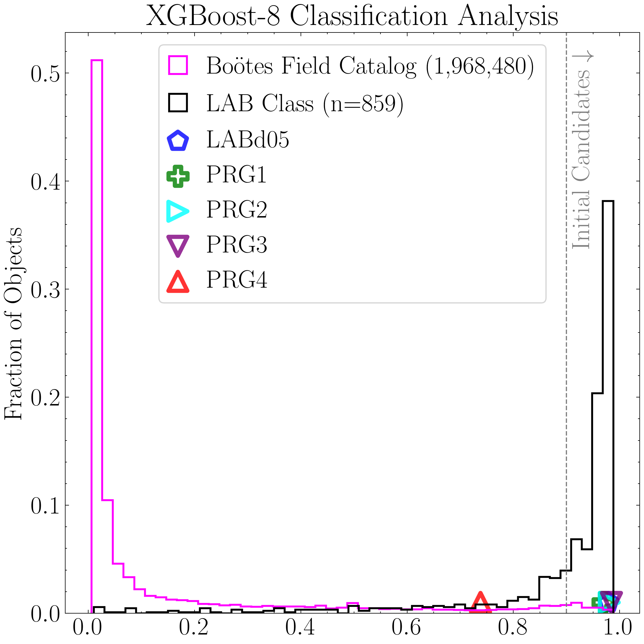
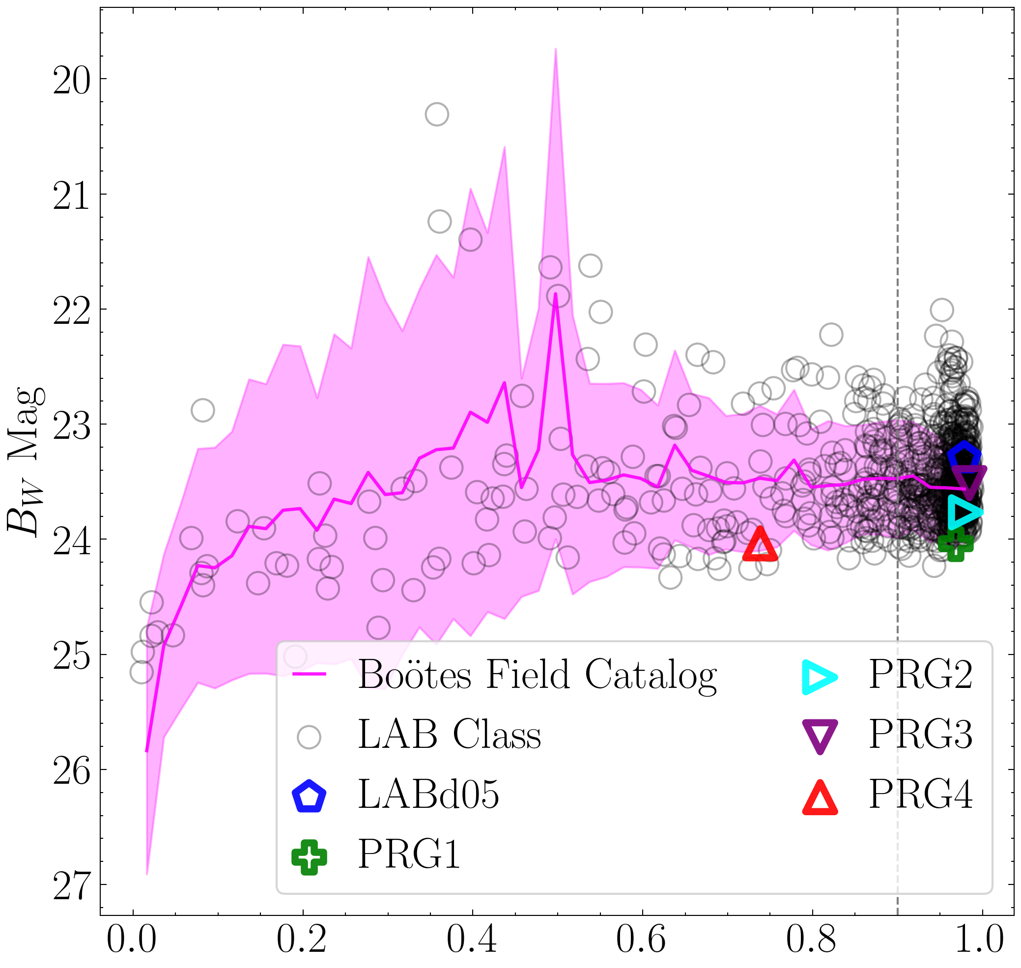
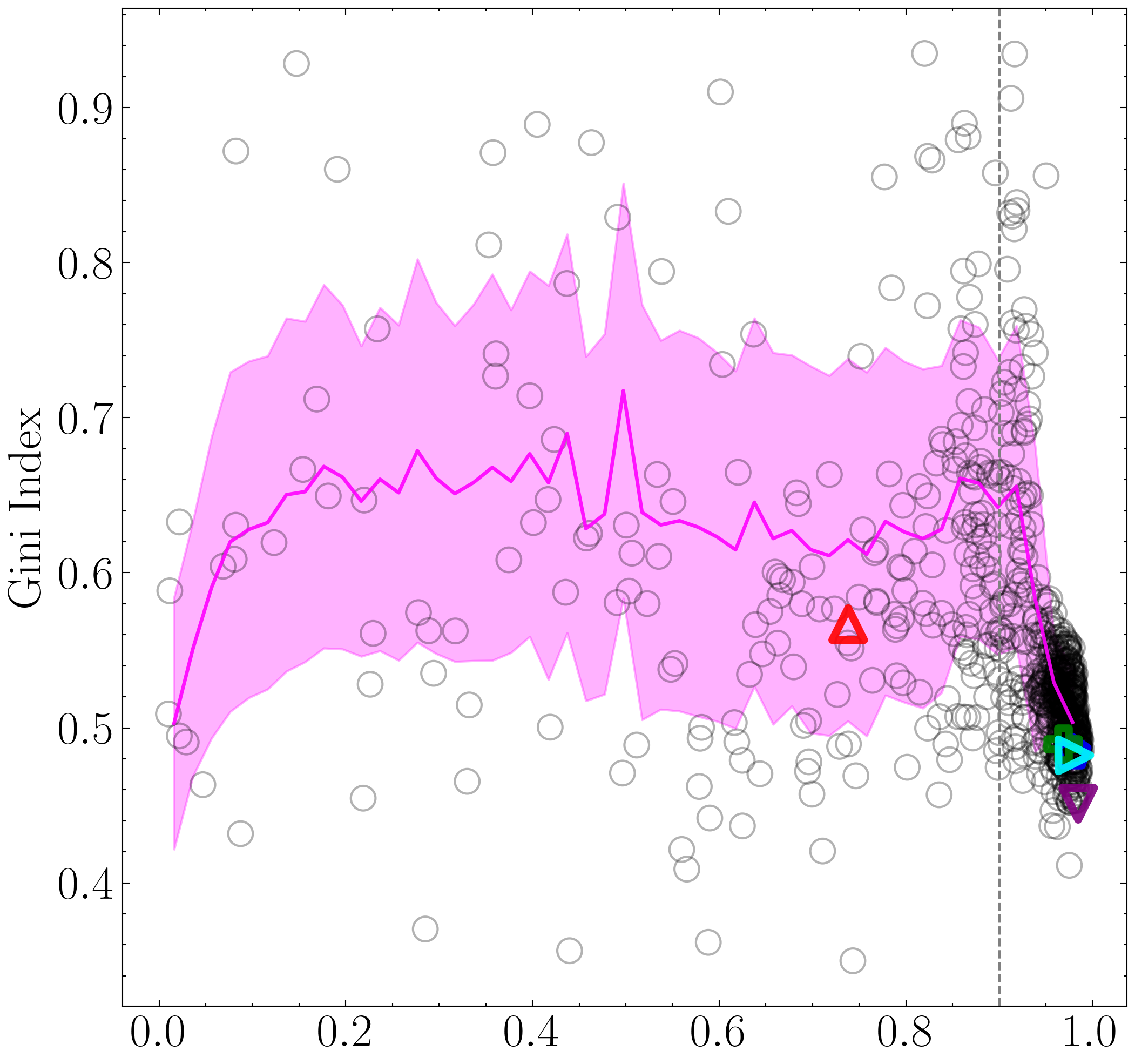
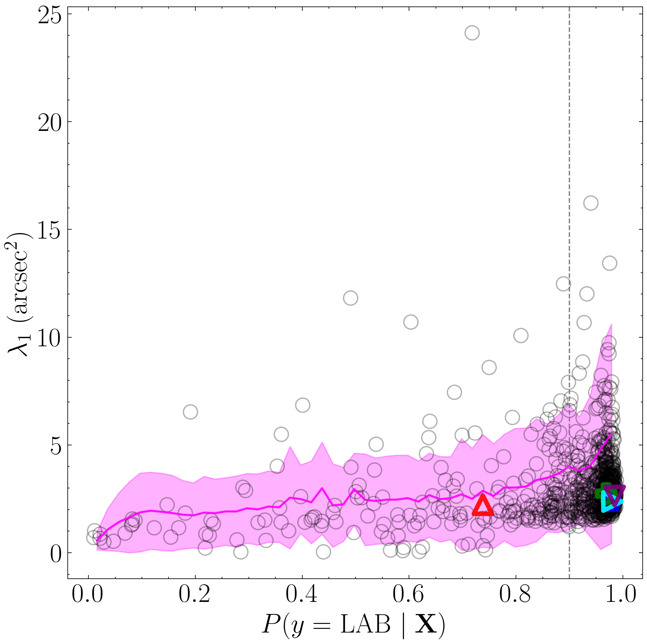
Image Extraction
To prepare for training the outlier-detection algorithm and the CNN, we now extract the multi-band imaging of our initial candidates, which includes only those with XGBoost probability predictions greater than or equal to 0.9.
This step requires two supporting files: (1) the catalog names of the 80 priority candidates in our training sample (from Prescott et al 2012), and (2) the names of the training-set LABs with unusable R-band imaging, as these are excluded from both outlier detection and CNN training. These files can be downloaded below:
import os
import numpy as np
import pandas as pd
from astropy.io import fits
from astropy.stats import SigmaClip
from photutils.aperture import ApertureStats, CircularAnnulus
from pyBIA.data_processing import crop_image, concat_channels

# Extract Other Images First #

# First the images are saved as individual files (for ease of processing, not needed and not provided in this documentation)
# Then these are loaded and compiled to form a single binary file (this is what is needed, and provided in this documentation)

# Where the images will be saved (as txt files)
bw_images_path = 'OTHER/Bw/'
r_images_path = 'OTHER/R/'

# The path to the NDWFS data files
data_path_bw = 'NDWFS/fits_images/Bw_FITS/'
data_path_r = 'NDWFS/fits_images/R_FITS/'

# Load the candidate catalog according to the optimized model
cat = pd.read_csv('candidate_catalog_optimized_xgboost_8.csv')

# Select only the candidates with probability predictions greater than or equal to 90%
index = np.where(cat.proba >= 0.90)[0]
sample = cat.iloc[index]

# Saving images as 250x250 pix
image_size = 250

# Setting the apertures for the background subtraction, approximated using the sigma-clipped median within annuli of 20 and 35 pixel radii
annulus_apertures = CircularAnnulus((int(image_size/2), int(image_size/2)), r_in=20, r_out=35)

# Extract the images one field at a time, normalizing by the exposure time to convert to counts per second
counter = 0
for field_name in np.unique(sample['field_name']):

        # Load the Bw and R broadband data
        hdu_bw = fits.open(data_path_bw+field_name+'_Bw_03_fix.fits')
        hdu_r = fits.open(data_path_r+field_name+'_R_03_reg_fix.fits')

        # Select only the objects in this subfield
        subfield_index = np.where(sample['field_name'] == field_name)[0]

        # Loop through these objects, subtract the background using aperture photometry, and save as txt file
        for i in range(len(subfield_index)):

                counter += 1
                print(counter)

                # Select the object's pixel positions
                xpix, ypix = sample[['xpix', 'ypix']].iloc[subfield_index[i]].values.T

                # Bw first, crop the image from the entire subfield array, and calculate the background in this region
                image = crop_image(hdu_bw[0].data, x=np.array(xpix), y=np.array(ypix), size=image_size, invert=True)
                bkg_stats = ApertureStats(image, annulus_apertures, error=None, sigma_clip=SigmaClip())

                # Subtract the background and then normalize by the exposure time to get counts/sec
                image = (image - bkg_stats.median) / hdu_bw[0].header['EXPTIME']
                np.savetxt(bw_images_path+sample.obj_name.iloc[subfield_index[i]], image)

                # R next, crop the image from the entire subfield array, and calculate the background in this region
                image = crop_image(hdu_r[0].data, x=np.array(xpix), y=np.array(ypix), size=image_size, invert=True)
                bkg_stats = ApertureStats(image, annulus_apertures, error=None, sigma_clip=SigmaClip())

                # Subtract the background and then normalize by the exposure time to get counts/sec
                image = (image - bkg_stats.median) / hdu_r[0].header['EXPTIME']
                np.savetxt(r_images_path+sample.obj_name.iloc[subfield_index[i]], image)

# Load the object names that were saved
obj_names = [name for name in os.listdir(bw_images_path) if 'NDWFS' in name]

# To store the Bw images and save as a single binary file
images = []
for name in obj_names:
        Bw = np.loadtxt(bw_images_path+name)
        images.append(Bw)

# Save the Bw images, this is what we provide in this documentation
np.save('xgb_output_images_bw.npy', np.array(images))

# To store the R images and save as a single binary file
images = []
for name in obj_names:
        R = np.loadtxt(r_images_path+name)
        images.append(R)

# Save the R images, this is what we provide in this documentation
np.save('xgb_output_images_R.npy', np.array(images))

# Save the corresponding names
np.savetxt('xgb_output_images_names.txt', obj_names, fmt='%s')

### Now extract the training set LAB Images ###

#Note: All 860 are saved which includes the singular non-detection as this is still useful for outlier detection

# Where the images will be saved (as txt files, for ease of processing, not needed and not provided in this documentation)
confirmed_diffuse_images_path_bw = 'LAB_images/confirmed_diffuse/Bw/'
priority_diffuse_images_path_bw = 'LAB_images/priority_diffuse/Bw/'
other_diffuse_images_path_bw = 'LAB_images/other_diffuse/Bw/'

confirmed_diffuse_images_path_r = 'LAB_images/confirmed_diffuse/R/'
priority_diffuse_images_path_r = 'LAB_images/priority_diffuse/R/'
other_diffuse_images_path_r = 'LAB_images/other_diffuse/R/'

# Where the training set files were saved
nsig_path = 'nsigs/'

# The training set file
sig = 0.32 #The optimal sig threshold to apply as per Figure 2
sample = pd.read_csv(f'{nsig_path}_Bw_training_set_nsig_{sig}')

# Identify the diffuse objects from the training set
diffuse_index = np.where(sample.flag == 1)[0] #Includes all 860 objects therefore includes the singular non-detection
names_to_save = np.array(sample.obj_name.iloc[diffuse_index])

# The names of the objects for which there is no R-band data or the data quality in this filter is bad
bad_r_names = np.loadtxt('bad_r_names_866.txt', dtype=str)

names_to_save = [i for i in names_to_save if i not in bad_r_names]

# Will identify the priority candidates as selected by Prescott et al. (2012), so as to save separately
obj_names_80 = np.loadtxt('obj_name_80', dtype=str)

# Will also save the five confirmed blobs separately
obj_names_5 = np.loadtxt('confirmed_LAB_names.txt', dtype=str)

# Saving images as 250x250 pix
image_size = 250

# Setting the apertures for the background subtraction, approximated using the sigma-clipped median within annuli of 20 and 35 pixel radii
annulus_apertures = CircularAnnulus((int(image_size/2), int(image_size/2)), r_in=20, r_out=35)

for field_name in np.unique(sample['field_name']):

        # Load the B and R broadband data
        hdu_bw = fits.open(data_path_bw+field_name+'_Bw_03_fix.fits')
        hdu_r = fits.open(data_path_r+field_name+'_R_03_reg_fix.fits')

        # Select only the objects in this subfield
        subfield_index = np.where(sample['field_name'] == field_name)[0]

        # Loop through these objects, subtract the background using aperture photometry, and save as txt file
        for i in range(len(subfield_index)):

                if sample.obj_name.iloc[subfield_index[i]] in names_to_save:

                        xpix, ypix = sample[['xpix', 'ypix']].iloc[subfield_index[i]].values.T

                        # Bw first, crop the image from the entire subfield array, and save the bkg subtracted sub-array
                        image = crop_image(hdu_bw[0].data, x=np.array(xpix), y=np.array(ypix), size=image_size, invert=True)
                        bkg_stats = ApertureStats(image, annulus_apertures, error=None, sigma_clip=SigmaClip())

                        # Subtract the background and then normalize by the exposure time to get counts/sec
                        image = (image - bkg_stats.median) / hdu_bw[0].header['EXPTIME']

                        if sample.obj_name.iloc[subfield_index[i]] in obj_names_80:
                                np.savetxt(priority_diffuse_images_path_bw+sample.obj_name.iloc[subfield_index[i]], image)
                        elif sample.obj_name.iloc[subfield_index[i]] in obj_names_5:
                                np.savetxt(confirmed_diffuse_images_path_bw+sample.obj_name.iloc[subfield_index[i]], image)
                        else:
                                np.savetxt(other_diffuse_images_path_bw+sample.obj_name.iloc[subfield_index[i]], image)

                        # R next, crop the image from the entire subfield array, and save the bkg subtracted sub-array
                        image = crop_image(hdu_r[0].data, x=np.array(xpix), y=np.array(ypix), size=image_size, invert=True)
                        bkg_stats = ApertureStats(image, annulus_apertures, error=None, sigma_clip=SigmaClip())

                        # Subtract the background and then normalize by the exposure time to get counts/sec
                        image = (image - bkg_stats.median) / hdu_r[0].header['EXPTIME']
                        if sample.obj_name.iloc[subfield_index[i]] in obj_names_80:
                                np.savetxt(priority_diffuse_images_path_r+sample.obj_name.iloc[subfield_index[i]], image)
                        elif sample.obj_name.iloc[subfield_index[i]] in obj_names_5:
                                np.savetxt(confirmed_diffuse_images_path_r+sample.obj_name.iloc[subfield_index[i]], image)
                        else:
                                np.savetxt(other_diffuse_images_path_r+sample.obj_name.iloc[subfield_index[i]], image)

# Save the five confirmed diffuse as a single binary file (this is what we provide in this documentation)
obj_names_confirmed_diffuse = [name for name in os.listdir(confirmed_diffuse_images_path_bw) if 'NDWFS' in name]

images = []
for name in obj_names_confirmed_diffuse:
        Bw, R = np.loadtxt(confirmed_diffuse_images_path_bw+name), np.loadtxt(confirmed_diffuse_images_path_r+name)
        images.append(concat_channels(Bw, R))

np.save('confirmed_diffuse.npy', np.array(images))
np.savetxt('confirmed_diffuse_names.txt', obj_names_confirmed_diffuse, fmt='%s')

# Save the 80 priority diffuse candidates as a single binary file (this is what we provide in this documentation)
obj_names_priority_diffuse = [name for name in os.listdir(priority_diffuse_images_path_bw) if 'NDWFS' in name]

images = []
for name in obj_names_priority_diffuse:
        Bw, R = np.loadtxt(priority_diffuse_images_path_bw+name), np.loadtxt(priority_diffuse_images_path_r+name)
        images.append(concat_channels(Bw, R))

np.save('priority_diffuse.npy', np.array(images))
np.savetxt('priority_diffuse_names.txt', obj_names_priority_diffuse, fmt='%s')

# Save the other diffuse candidates as a single binary file (this is what we provide in this documentation)
obj_names_other_diffuse = [name for name in os.listdir(other_diffuse_images_path_bw) if 'NDWFS' in name]

images = []
for name in obj_names_other_diffuse:
        Bw, R = np.loadtxt(other_diffuse_images_path_bw+name), np.loadtxt(other_diffuse_images_path_r+name)
        images.append(concat_channels(Bw, R))

np.save('other_diffuse.npy', np.array(images))
np.savetxt('other_diffuse_names.txt', obj_names_other_diffuse, fmt='%s')
The candidate images in binary format (containing approximately 50,000 objects), along with their catalog names, are available for download below:
The LAB training-set images in binary format, along with their catalog names, are available for download below.
Images:
Corresponding names:
Outlier Removal
We find that a subset of classified objects are outliers (e.g., edge effects, bright halos contaminating the pixel distribution, or bleed trails from nearby stars). After visually inspecting a subset of candidates, we manually selected 1,000 objects identified as outliers in either band. These are available for download as a binary file along with the corresponding catalog names:
We begin by plotting four of these outliers using the plot_images_grid_2x2 function provided in the Catalog module.
import numpy as np
from pyBIA import catalog

images = np.load('outlier_sample_visually_inspected.npy')
images = images[:,:,:,0] # Only show the Bw

pix_conversion = 3.8961 # NDWFS survey pixel-per-arcsecond (for setting the axes)
size = 250 # Will crop the image to be of this size, otherwise set to None
xpix = ypix = images.shape[1] // 2 # Cropped image will be centered about these coords, if not cropping set to None
suptitle = r'Example Outliers ($B_W$)'

# Plot the first three images and the tenth one for variety
savepath = f'example_outliers.png'
catalog.plot_images_grid_2x2(
        images[0],
        images[1],
        images[2],
        images[10],
        pix_conversion=pix_conversion,
        suptitle=suptitle,
        xpix=xpix,
        ypix=ypix,
        size=size,
        savepath=savepath
        )
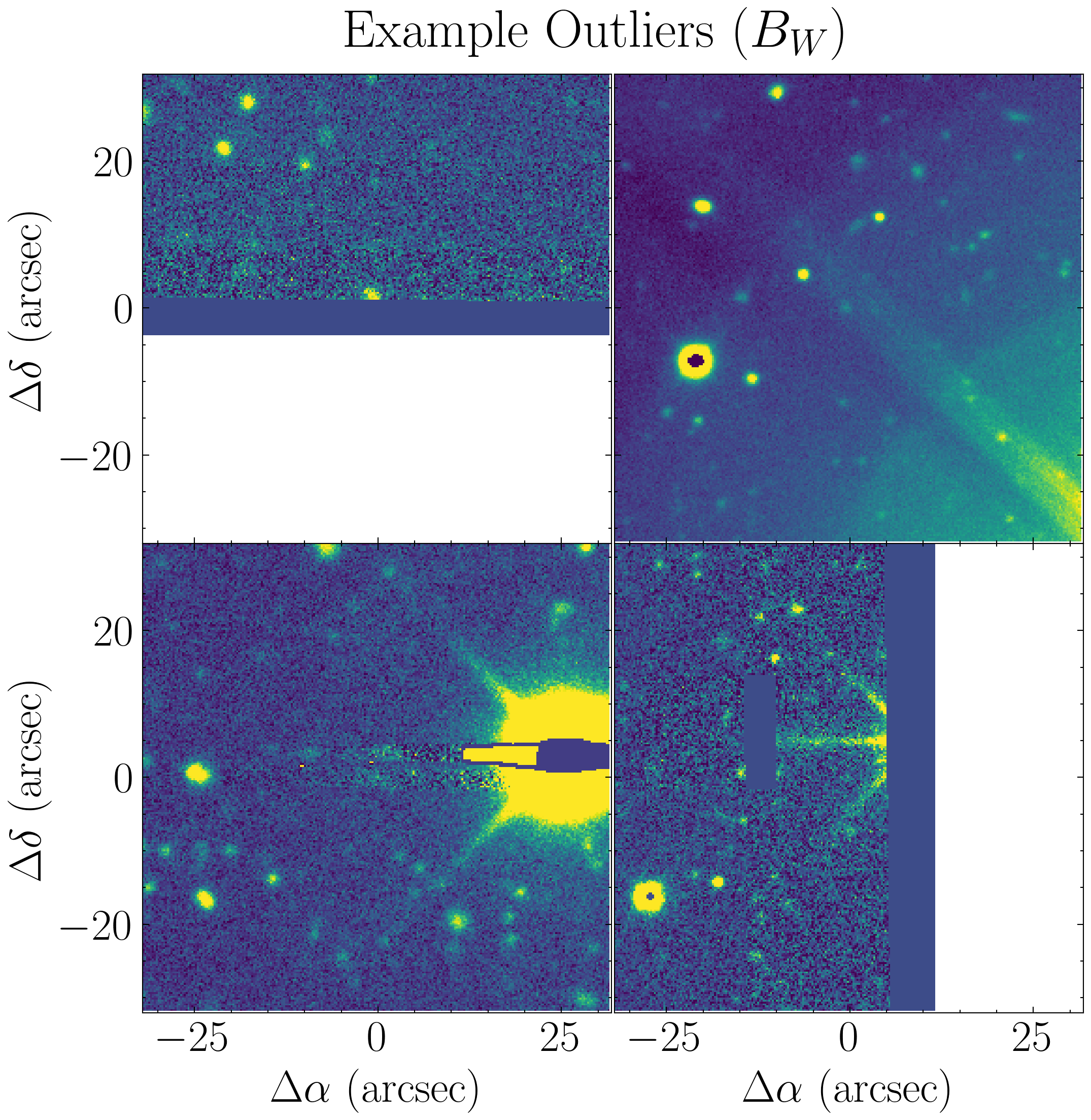
To detect such outliers, we train a multi-band Isolation Forest (iForest) model on the LAB class. We reserve 100 LABs for testing and evaluate performance by measuring the model’s ability to correctly classify these 100 as inliers while simultaneously identifying the 1,000 visually confirmed outliers described above.
In this work, we test five distinct feature sets for iForest training and vary the image cutout size to determine the optimal dimensions for model performance.
This analysis is performed using the outlier_detection module.
import numpy as np
from pyBIA.data_augmentation import resize
from pyBIA import outlier_detection

# We experiment with square image sizes with lengths between 50 and 250 pixels
image_sizes = np.arange(50, 251, 1)

normalize = True # Whether to min-max normalize the images
min_pixel = 0 # Min pixel for min-max normalization
max_pixel = 10 # Max pixel for min-max normalization
img_num_channels = 2 # Number of channels
clf = 'iforest' # Model to use, code only supports iForest at the moment
impute = True # Whether to impute missing data
imp_method = 'median' # Imputation method
SEED_NO = 1909 # Random seed for training the iForest model

# Extract the features for the positive class (all DIFFUSE training objects)
for image_size in image_sizes:

        print(image_size)

        # Load the LAB training set images saved during image extraction
        confirmed_LAB = np.load('confirmed_diffuse.npy') # 5 confirmed
        priority_LAB = np.load('priority_diffuse.npy') # 80 priority
        other_LAB =  np.load('other_diffuse.npy') #760 other diffuse

        # Combine and resize
        all_LAB = np.vstack((confirmed_LAB, priority_LAB, other_LAB))
        all_LAB = resize(all_LAB, image_size)

        # Set the data used for training and testing, shuffle first since theyre ordered according to priority
        rng = np.random.default_rng(seed=SEED_NO)
        shuffled_indices = rng.permutation(len(all_LAB))
        all_LAB = all_LAB[shuffled_indices]
        LAB_train = all_LAB[:745]
        LAB_test = all_LAB[745:]

        # Load the outliers we will use to test the performance
        selected_outliers = np.load('outlier_sample_visually_inspected.npy')
        selected_outliers = selected_outliers
        selected_outliers = resize(selected_outliers, image_size)

        # Loop through the different feature sets and save the results in a dir called Outlier_Detection
        for feat_set in ['hog', 'wavelet', 'stats', 'lbp', 'fft']:

                # Instantiate the classifier
                model = outlier_detection.Classifier(
                        data=LAB_train,
                        normalize=normalize,
                        min_pixel=min_pixel,
                        max_pixel=max_pixel,
                        img_num_channels=img_num_channels,
                        feat_set=feat_set,
                        clf=clf,
                        impute=impute,
                        imp_method=imp_method,
                        SEED_NO=SEED_NO
                        )

                # Train the classifier
                model.create()

                # Predict on the test sets
                predictions_LAB_test = model.predict(LAB_test)
                predictions_outliers = model.predict(selected_outliers)

                # Save test set prediction results
                np.savetxt(f'Outlier_Detection/LAB/{feat_set.upper()}/pred_LAB_{image_size}pix.txt', predictions_LAB_test, header='predictions, decision_function_scores, raw_anomaly_scores')
                np.savetxt(f'Detection/outliers/{feat_set.upper()}/pred_outliers_{image_size}pix.txt', predictions_outliers, header='predictions, decision_function_scores, raw_anomaly_scores')
The directory containing the test-set results as a function of image size and feature set can be downloaded here.
We now proceed to plot the model performance as a function of both image size and feature set.
import numpy as np
import matplotlib.pyplot as plt
import scienceplots
plt.style.use('science')
plt.rcParams.update({'font.size': 21, 'lines.linewidth': 1.5})

pix_conversion = 3.8961 # NDWFS pix-to-arcsec conversion factor
image_sizes = np.arange(50, 251, 1) # Image sizes we tested

# Convert to physical units
image_sizes_arcsec = image_sizes / pix_conversion

# The five feature sets used in analysis
feature_sets = ['HOG', 'WAVELET', 'LBP', 'FFT', 'STATS']

# Legend label mapping
feature_label_map = {
    'HOG': 'HOG',
    'WAVELET': 'Wavelet',
    'STATS': 'Stats',
    'LBP': 'LBP',
    'FFT': 'FFT'
}

colors = plt.cm.tab10.colors
linestyles = ['-', '--', '-.', ':', (0, (4, 2, 1, 2, 1, 2))]

# Load outlier detection rates, from directory provided above
detection_rates = {feat: [] for feat in feature_sets}
base_path_out = 'Outlier_Detection/outliers'

for feat in feature_sets:
    for size in image_sizes:
        preds = np.loadtxt(f'{base_path_out}/{feat}/pred_outliers_{size}pix.txt')[:, 0]
        rate = np.mean(preds == -1)
        detection_rates[feat].append(rate)

# Find optimal
max_val = -1
max_feat = None
max_size = None
for feat in feature_sets:
    for size, val in zip(image_sizes, detection_rates[feat]):
        if val > max_val:
            max_val = val
            max_feat = feat
            max_size = size

max_arcsec = max_size / pix_conversion

# Load inlier detection rates, from directory provided above
retention_rates = {feat: [] for feat in feature_sets}
base_path_in = 'Outlier_Detection/LAB'

for feat in feature_sets:
    for size in image_sizes:
        preds = np.loadtxt(f'{base_path_in}/{feat}/pred_LAB_{size}pix.txt')[:, 0]
        rate = np.mean(preds == 1)
        retention_rates[feat].append(rate)

# Plot
fig, (ax1, ax2) = plt.subplots(2, 1, figsize=(8, 16), sharex=True)
fig.subplots_adjust(top=0.9, hspace=0.02)  # reduced space between plots

# Plot the outlier detection rates
for i, feat in enumerate(feature_sets):
    ax1.plot(image_sizes_arcsec, detection_rates[feat], label=feature_label_map[feat],
             linewidth=2.5, color=colors[i % 10], linestyle=linestyles[i % len(linestyles)])

ax1.axvline(max_arcsec, linestyle=(0, (2, 2)), alpha=0.7, color='gray')
ax1.annotate(
    f"Optimal\n(HOG)",
    xy=(max_arcsec, max_val),
    xytext=(-17.4, -340),
    textcoords="offset points",
    ha="right", va="top", color="gray",
    rotation=90, rotation_mode="anchor", fontsize=18,
)
ax1.set_ylabel('Outlier Detection Rate')
ax1.set_xlim((image_sizes_arcsec.min(), image_sizes_arcsec.max()))
ax1.set_title('iForest Performance', y=1.15)

# Plot the inlier detection rates
for i, feat in enumerate(feature_sets):
    ax2.plot(image_sizes_arcsec, retention_rates[feat],
             linewidth=2.5, color=colors[i % 10], linestyle=linestyles[i % len(linestyles)])

ax2.axvline(max_arcsec, linestyle=(0, (2, 2)), alpha=0.7, color='gray')
ax2.set_ylabel('Inlier Detection Rate')
ax2.set_xlabel('Image Size (arcsec)')

handles, labels = ax1.get_legend_handles_labels()
fig.legend(handles, labels, loc='upper center', bbox_to_anchor=(0.5, 0.968), ncol=5,
           title='Feature Set', frameon=True, fancybox=True, handlelength=1.2,
           columnspacing=0.7, handletextpad=0.5)

plt.savefig('combined_outlier_inlier_vs_size_arcsec.png', dpi=300, bbox_inches='tight')
plt.show()
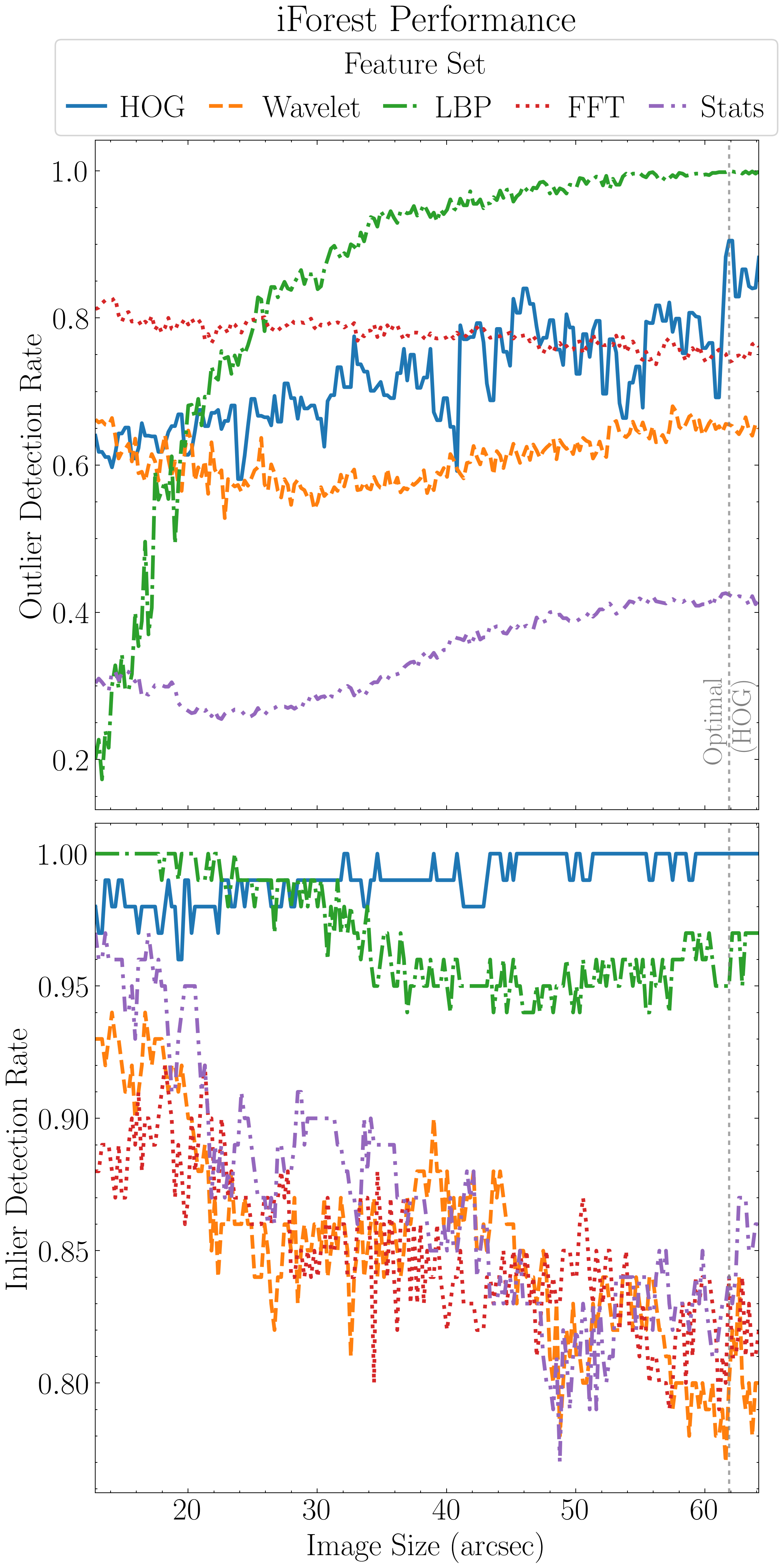
After determining the best feature set (HOG features) and the optimal image size (241×241 pixels), we proceed with training and saving the the optimal iForest model and classifying the initial candidates to flag any outliers present.
For this we load the previously saved binary files xgb_output_images_bw.npy and xgb_output_images_R.npy, which contain the imaging data for all initial candidate objects (approximately 53,000). After classifying these, we save the anomaly detection scores alongside several Bw-based morphological features from the image segmentation routine conducted earlier. These include the area of the segmentation patch as well as the first eigenvalue of the covariance matrix.
import numpy as np
import pandas as pd
from pyBIA import outlier_detection
from pyBIA.data_processing import concat_channels
from pyBIA.data_augmentation import resize

image_size = 241 # Optimal image size to use
normalize = True # Whether to min-max normalize the images
min_pixel = 0 # Min pixel for min-max normalization
max_pixel = 10 # Max pixel for min-max normalization
img_num_channels = 2 # Number of channels
feat_set = 'hog' # Optimal feature set to use
clf = 'iforest' # Model to use, code only supports iForest at the moment
impute = True # Whether to impute missing data
imp_method = 'median' # Imputation method
SEED_NO = 1909 # Random seed for training the iForest model

# Train and save the optimal model now that we know best feature set and image size to use
confirmed_LAB = np.load('confirmed_diffuse.npy') # 5 confirmed
priority_LAB = np.load('priority_diffuse.npy') # 80 priority
other_LAB =  np.load('other_diffuse.npy') #760 other diffuse

# Combine and resize
all_LAB = np.vstack((confirmed_LAB, priority_LAB, other_LAB))
all_LAB = resize(all_LAB, image_size)

# Same shuffling and test partitioning as during the previous analysis
rng = np.random.default_rng(seed=SEED_NO)
shuffled_indices = rng.permutation(len(all_LAB))
all_LAB = all_LAB[shuffled_indices]
LAB_train = all_LAB[:745]

# Instantiate the classifier
model = outlier_detection.Classifier(
        data=LAB_train,
        normalize=normalize,
        min_pixel=min_pixel,
        max_pixel=max_pixel,
        img_num_channels=img_num_channels,
        feat_set=feat_set,
        clf=clf,
        impute=impute,
        imp_method=imp_method,
        SEED_NO=SEED_NO
        )

# Create and save the model inside a folder called anomaly_detection_model
model.create()
model.save(dirname='anomaly_detection_model')

# CLASSIFY ALL THE CANDIDATES TO IDENTIFY THE OUTLIERS #

# We do this in several batches for ease of processing
prediction_candidates = []
for i in range(4):

        other_bw = np.load('xgb_output_images_bw.npy')
        other_r = np.load('xgb_output_images_R.npy')

        #Index 15k at a time
        other_bw = other_bw[i*15000:(i+1)*15000] #15k at a time
        other_r = other_r[i*15000:(i+1)*15000]

        # Combine and resize
        other = concat_channels(other_bw, other_r)
        other = resize(other, image_size)

        # Make the predictions and append
        iforest_predictions = model.predict(other)
        prediction_candidates.append(iforest_predictions)

# NOW STORE THE AREAS/COVAREIGVAL OF THE DETECTED OUTLIERS FOR ANALYSIS #

# Load the data we just saved (the Classifier class outputs three values per preditiction, classification + decision function score + anomaly score)
iforest_preds = np.vstack(prediction_candidates)
preds, decision_scores, anomaly_scores = iforest_preds[:,0], iforest_preds[:,1], iforest_preds[:,2]

# Load the names of the initial candidates
candidate_names = np.loadtxt('xgb_output_images_names.txt', dtype=str)

#Load the candidate catalog
cat = pd.read_csv('candidate_catalog_optimized_xgboost_8.csv')

# Find the areas and first eigenvalue of the covariance matrix
areas, lambda_1 = [], []

for i in range(len(candidate_names)):
        index = np.where(cat.obj_name == candidate_names[i])[0]
        areas.append(cat.area.iloc[int(index)])
        lambda_1.append(cat.covariance_eigval1.iloc[int(index)])

np.savetxt('outlier_scores_and_areas.txt', np.c_[candidate_names, preds, decision_scores, anomaly_scores, areas, lambda_1], header='candidate_names, preds, decision_scores, anomaly_scores, areas, lambda_1', fmt='%s')
The pyBIA iForest model can be downloaded here.
The saved predictions for the candidate objects, along with their corresponding area and the first eigenvalue of the covariance matrix, can be downloaded here.
With the predictions and morphological values saved, we can now generate the figure showing the iForest score distributions and the correlation between the scores and the effective extent of the image-segmentation patches.
import numpy as np
import matplotlib.pyplot as plt
import scienceplots
plt.style.use('science')
plt.rcParams.update({'font.size': 21, 'lines.linewidth': 1.5})

image_size = 241 # Optimal image size

# Load inlier and outlier decision scores from previous analysis (see saved directory above)
outlier_scores = np.loadtxt(f'Outlier_Detection/outliers/HOG/pred_outliers_{image_size}pix.txt')
outlier_anomaly_scores = outlier_scores[:, 1]

inlier_scores = np.loadtxt(f'Outlier_Detection/LAB/HOG/pred_LAB_{image_size}pix.txt')
inlier_anomaly_scores = inlier_scores[:, 1]

# Load Initial Candidates
data = np.loadtxt('outlier_scores_and_areas.txt', dtype=str)
initial_scores = data[:, 2].astype(float)

pix_conversion = 3.8961 # NDWFS Bootes field pix-to-arcsec conversion

# Common bins
all_scores = np.concatenate([outlier_anomaly_scores, inlier_anomaly_scores, initial_scores])
num_bins = 30
bins = np.linspace(all_scores.min(), all_scores.max(), num_bins + 1)
bin_centers = 0.5 * (bins[:-1] + bins[1:])

# Histograms
hist_out, _ = np.histogram(outlier_anomaly_scores, bins=bins)
hist_in, _ = np.histogram(inlier_anomaly_scores, bins=bins)
hist_init, _ = np.histogram(initial_scores, bins=bins)

frac_out = hist_out / np.sum(hist_out)
frac_in = hist_in / np.sum(hist_in)
frac_init = hist_init / np.sum(hist_init)

# Morphological attributes
feat_to_plot = 'area'
second_feat = 'covariance_eigval1'
scores, areas, lambda_1 = data[:, 2].astype(float), data[:, 4].astype(float), data[:, 5].astype(float)

def get_feat(name):
    # Convert to physical units
    if name == 'area':
        return np.array(areas) / pix_conversion**2, r'$B_W$ Area (arcsec$^2$)'
    elif name == 'covariance_eigval1':
        return np.array(lambda_1) / pix_conversion**2, r'$\lambda_1$ (arcsec$^2$)'

feat, ylabel = get_feat(feat_to_plot)
if second_feat:
    second, ylabel2 = get_feat(second_feat)

bin_indices = np.digitize(scores, bins) - 1
mean_feat = np.array([np.nanmean(feat[bin_indices == i]) if np.any(bin_indices == i) else np.nan for i in range(len(bins)-1)])
std_feat = np.array([np.nanstd(feat[bin_indices == i]) if np.any(bin_indices == i) else np.nan for i in range(len(bins)-1)])

if second_feat:
    mean_second = np.array([np.nanmean(second[bin_indices == i]) if np.any(bin_indices == i) else np.nan for i in range(len(bins)-1)])
    std_second = np.array([np.nanstd(second[bin_indices == i]) if np.any(bin_indices == i) else np.nan for i in range(len(bins)-1)])

# Plot
fig, (ax1, ax2) = plt.subplots(2, 1, figsize=(8, 16), sharex=True, gridspec_kw={'hspace': 0.022})

# Top panel
ax1.step(bin_centers, frac_in, where='mid', linestyle='-', label=f'Inliers (n={len(inlier_anomaly_scores)})', linewidth=2.5)
ax1.step(bin_centers, frac_out, where='mid', linestyle='--', label=f'Outliers (n={len(outlier_anomaly_scores)})', linewidth=2.5)
ax1.step(bin_centers, frac_init, where='mid', linestyle='-.', label=f'Initial Candidates (n={len(initial_scores):,})', linewidth=2.5, color='magenta')
ax1.set_ylabel('Fraction of Objects')
ax1.set_title('Optimal iForest Model')
ax1.legend(frameon=True, fancybox=True)
ax1.set_xlim(bin_centers[0], bin_centers[-1])
ax1.set_ylim(0)
ax1.axvline(0.0, linestyle=(0, (2, 2)), alpha=0.7, color='gray')
ax1.annotate(r'Outliers $\uparrow$', xy=(0.0, 0.11), xytext=(-18, 0),
             textcoords='offset points', ha='left', va='bottom', color='gray', rotation=90)

# Lower panel
line1 = ax2.plot(bin_centers, mean_feat, linestyle='-', linewidth=2.5, color='tab:blue', label=r'$\lambda_1$')
ax2.fill_between(bin_centers, mean_feat - std_feat, mean_feat + std_feat, color='tab:blue', alpha=0.3)
ax2.set_xlabel('Score')
ax2.set_ylabel(ylabel)

if second_feat:
    ax2b = ax2.twinx()
    line2 = ax2b.plot(bin_centers, mean_second, linestyle='--', linewidth=2.5, color='tab:red', label='Area')
    ax2b.fill_between(bin_centers, mean_second - std_second, mean_second + std_second, color='tab:red', alpha=0.2)
    ax2b.set_ylabel(ylabel2)
    lines = line2 + line1
    labels = [l.get_label() for l in lines]
    ax2.legend(lines, labels, frameon=True, fancybox=True)

ax2.set_xlim(bin_centers[0], bin_centers[-1])
ax2.set_ylim(0)
ax2.axvline(0.0, linestyle=(0, (2, 2)), alpha=0.7, color='gray')

plt.savefig('iforest_scores.png', dpi=300, bbox_inches='tight')
plt.show()
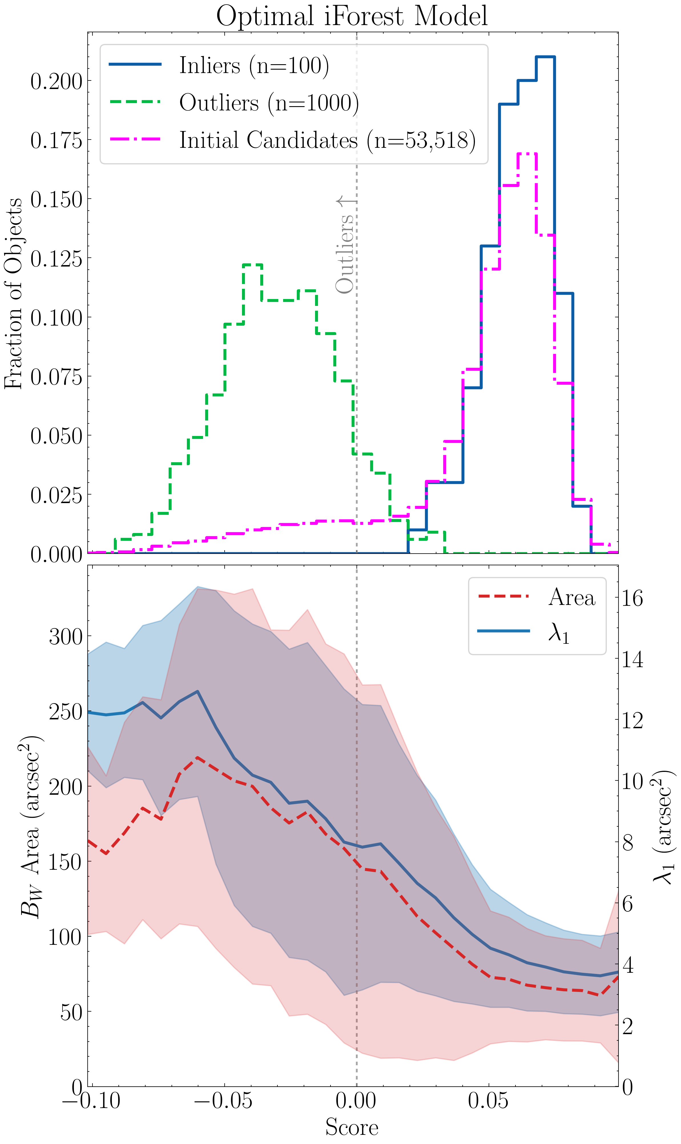
CNN Training
With the majority of outliers removed from the candidate sample, we now train the multi-band CNN to identify the most promising LAB candidates.
We begin by extracting the training-set images. The positive class consists of the 70 Prescott et al 2012 priority candidates classified by our XGBoost model with a probability greater than or equal to 0.9. The five confirmed LABs are reserved for testing. At the same time, we save the non-priority LABs from our training set that also made it through the pipeline, so that after CNN training, we can identify which of these should be considered final candidates. For computational efficiency, we also extract 3,800 random objects from our initial candidate sample to form the negative class.
import numpy as np
from pyBIA.data_processing import concat_channels

# Load the images provided during original image extraction
priority_lab_images = np.load('priority_diffuse.npy')
priority_lab_names = np.loadtxt('priority_diffuse_names.txt', dtype=str)

# Results for Leave-one-Out CV analysis
lab_loo = np.loadtxt('LoO_LAB', dtype=str)
lab_loo_names = lab_loo[:,0]
lab_loo_probas = lab_loo[:,2].astype('float') #xgboost-8 probas is the third column

names, probas = [],[]
for name in priority_lab_names:
        index = np.where(lab_loo_names == name)[0]
        names.append(name); probas.append(lab_loo_probas[index[0]])

# These are now aligned (i.e., names == priority_lab_names)
# Filter out those that did not have probability predictions of at least 0.9
index = np.where(np.array(probas) >= 0.9)[0]
priority_lab_images_final = priority_lab_images[index]
priority_lab_names_final = priority_lab_names[index]

np.save('priority_diffuse_final.npy', priority_lab_images_final)
np.savetxt('priority_diffuse_names_final.txt', priority_lab_names_final, fmt='%s')

# Now do the same for the non-priority LAB so after CNN training we can select the ones that are final candidates

# Load the images provided during original image extraction
other_lab_images = np.load('other_diffuse.npy')
other_lab_names = np.loadtxt('other_diffuse_names.txt', dtype=str)

# In this case not all the images have an associated proba, since there is one non-detection
# So have to loop over the names that have an xgboost-8 proba
names, probas = [],[]
for name in lab_loo_names:
        index = np.where(other_lab_names == name)[0]
        if len(index) == 0:
                pass
        else:
                names.append(name); probas.append(lab_loo_probas[index[0]])

# Finally query the images
indices = []
for i in range(len(names)):
        index = np.where(other_lab_names == names[i])[0]
        indices.append(index[0])

other_lab_images_final = other_lab_images[indices]
other_lab_names_final = other_lab_names[indices]

# Only need those that passed our initial XGBoost-based filtering
index = np.where(np.array(probas) >= 0.9)[0]
other_lab_images_final = other_lab_images_final[index]
other_lab_names_final = other_lab_names_final[index]

np.save('other_diffuse_final.npy', other_lab_images_final)
np.savetxt('other_diffuse_names_final.txt', other_lab_names_final, fmt='%s')

# Now save the training set for the initial candidates, only saving 3800 for CNN training purposes

# First find which ones made it through the iForest-based filtering (i.e., which ones are inliners)
candidate_names = np.loadtxt('xgb_output_images_names.txt', dtype=str)
outlier_data = np.loadtxt('iforest_predictions.txt')

ypred = outlier_data[:,0] # The prediction, 1 is inliers, -1 is outliers

# Now load the full image arrays saved previously
cand_bw = np.load('xgb_output_images_bw.npy')
cand_r = np.load('xgb_output_images_R.npy')

index = np.where(ypred == 1)[0] #Inliers
cand_bw = cand_bw[index]
cand_r = cand_r[index]
candidate_names = candidate_names[index]

# Random seed for random selection of training set objects
rng = np.random.default_rng(seed=1909)
shuffled_indices = rng.permutation(len(cand_bw))
shuffled_indices = shuffled_indices[:3800]

# Select only these 3800
cand_bw = cand_bw[shuffled_indices]
cand_r = cand_r[shuffled_indices]
candidate_names = candidate_names[shuffled_indices]

# Combine the filters
training_other = concat_channels(cand_bw, cand_r)

np.save('cnn_training_other_3800.npy', training_other)
np.savetxt('cnn_training_other_3800_names.txt', candidate_names, fmt='%s')
These files can be downloaded below.
Images:
Corresponding names:
With these images saved, we can now train our binary convolutional neural-network classifier using the cnn_model module.
import numpy as np
from pyBIA import cnn_model

# Load the negative class and add the third Bw-R difference channel
training_other = np.load('cnn_training_other_3800.npy')
training_bw_minus_r = training_other[:,:,:,0] / training_other[:,:,:,1]
training_bw_minus_r = np.expand_dims(training_bw_minus_r, axis=-1)
training_other = np.concatenate([training_other, training_bw_minus_r], axis=-1)

# 1000 used for testing filtering capabilities, the rest for training
testing_other = training_other[:1000]
training_other = training_other[1000:]

# Load the positive class and add the third Bw-R difference channel
train_lab_priority = np.load('priority_diffuse_final.npy')
lab_priority_bw_minus_r = train_lab_priority[:,:,:,0] / train_lab_priority[:,:,:,1]
lab_priority_bw_minus_r = np.expand_dims(lab_priority_bw_minus_r, axis=-1)
train_lab_priority = np.concatenate([train_lab_priority, lab_priority_bw_minus_r], axis=-1)

# Shuffle the training set before selecting valiation set just to be sure
rng = np.random.default_rng(seed=1909)
shuffled_indices = rng.permutation(len(train_lab_priority))
train_lab_priority = train_lab_priority[shuffled_indices]

# 56 positives used for training, 14 used for validation, so can do 5-fold CV
val_lab = train_lab_priority[:14]
train_lab = train_lab_priority[14:]

# Classifier class parameters
img_num_channels = 3 # Number of channels in our images
normalize = True # Whether to min-max normalize the pixels
min_pixel = 0 # Min pixel will be zero
max_pixel = [10,10,10] # Max pixel will be 10 for all three channels
clf = 'alexnet' # Architecture we will use
epochs = 6 # Number of epochs to train for
batch_size = 8 # Training batch size
opt_cv = 5 # Will do five-fold cross-validation
augment_data = True # Whether to apply data augmentation to the positive class
batch_positive = 24 # How many times to augment each positive instance
balance = True # Whether to downsample the negative class to match the positive
image_size = 70 # Will crop the images to be this size (applied to both classes post-data augmentation)
shift = 10 # The max allowed vertical/horizontal pixel shifts during data augmentation
rotation = horizontal = vertical = True # Whether to include rotations (0-360) and horizontal/vertical flips during data augmentation
activation_conv = 'relu' # Activation function for the Conv2D layers
activation_dense = 'tanh' # Activation function for the FC layers
model_reg = None # Regularized to use, options are 'local_response', 'batch_norm' or None
optimizer = 'adam' # Optimizer to use
lr = 0.00001 # Learning rate to use
amsgrad = True # Whether to enable the Adam AMSGrad variant
conv_init = 'he_normal' # Weight initilization scheme for the Conv2D layers
dense_init = 'glorot_uniform' # Weight initilization scheme for the FC layers

# Instantiate the classifier
model = cnn_model.Classifier(
        train_lab,
        training_other,
        val_positive=val_lab,
        val_negative=None,
        img_num_channels=img_num_channels,
        normalize=normalize,
        min_pixel=min_pixel,
        max_pixel=max_pixel,
        clf=clf,
        epochs=epochs,
        batch_size=batch_size,
        opt_cv=opt_cv,
        augment_data=augment_data,
        batch_positive=batch_positive,
        balance=balance,
        image_size=image_size,
        shift=shift,
        rotation=rotation,
        vertical=vertical,
        horizontal=horizontal,
        activation_conv=activation_conv,
        activation_dense=activation_dense,
        model_reg=model_reg,
        optimizer=optimizer,
        lr=lr,
        amsgrad=amsgrad,
        conv_init=conv_init,
        dense_init=dense_init)

# Create the model
model.create(overwrite_training=True)

# Save the pyBIA model
model.save(dirname='cnn_model')

# Test on the 1000 randomly selected
pred = model.predict(testing_other, target='LAB', return_proba=True, cv_model='all')
print('Fraction of sources classified as OTHER', len(np.where(pred[:,0]=='OTHER')[0])/len(pred))
The saved pyBIA model can be downloaded here.
We can then load this model and visualize its performance across epochs.
import numpy as np
from pyBIA import cnn_model
import matplotlib.pyplot as plt
import scienceplots
plt.style.use('science')
plt.rcParams.update({'font.size': 21})

model = cnn_model.Classifier()
model.load('cnn_model')

# Training metrics are saved in the following class attributes, shape is (num_folds, num_epochs, num_metrics)
train_metrics = np.array(model.model_train_metrics)
val_metrics = np.array(model.model_val_metrics)
epochs = np.arange(1, model.epochs + 1)

# Toggle this flag to switch between standard deviation and full range
use_full_range = False

def compute_range(metrics, use_full_range):
    # Compute mean with either standard deviation or full min-max range
    mean = np.mean(metrics, axis=0)
    if use_full_range:
        lower = np.min(metrics, axis=0) # Minimum across folds
        upper = np.max(metrics, axis=0) # Maximum across folds
    else:
        std = np.std(metrics, axis=0)
        lower = mean - std
        upper = mean + std
    return mean, lower, upper

# Plot the F1 score on top and Loss on bottom
fig, (ax1, ax2) = plt.subplots(2, 1, figsize=(8, 16), sharex=True)
fig.subplots_adjust(top=0.9, hspace=0.02)

column = 2 # F1 score in third column
column_val = 0 # The binary accuracy column, used only for the validation data
train_mean, train_lower, train_upper = compute_range(train_metrics[:, :, column], use_full_range)
val_mean, val_lower, val_upper = compute_range(val_metrics[:, :, column_val], use_full_range)

ax1.plot(epochs, train_mean, marker='o', color='blue', label='Training (F1 Score)')
ax1.fill_between(epochs, train_lower, train_upper, color='blue', alpha=0.3)
ax1.plot(epochs, val_mean, marker='s', linestyle='dashed', color='red', label='Validation (LAB Recall)')
ax1.fill_between(epochs, val_lower, val_upper, color='red', alpha=0.3)

ax1.set_ylabel('Score')
ax1.set_title('CNN Model Training Results (5-Fold CV)', y=1.095)

column = 1 # Loss in second column
train_mean, train_lower, train_upper = compute_range(train_metrics[:, :, column], use_full_range)
val_mean, val_lower, val_upper = compute_range(val_metrics[:, :, column], use_full_range)

ax2.plot(epochs, train_mean, marker='o', color='blue', label='Training Set')
ax2.fill_between(epochs, train_lower, train_upper, color='blue', alpha=0.3)
ax2.plot(epochs, val_mean, marker='s', linestyle='dashed', color='red', label='Validation Set')
ax2.fill_between(epochs, val_lower, val_upper, color='red', alpha=0.3)

ax2.set_ylabel('Loss')
ax2.set_xlabel('Epochs')

legend_title = r'5-Fold CV (Full Range)' if use_full_range else r'5-Fold CV ($\pm \sigma$)'
handles, labels = ax1.get_legend_handles_labels()
fig.legend(handles, labels, loc='upper center', bbox_to_anchor=(0.5, 0.945), ncol=2,
           frameon=True, fancybox=True, handlelength=1.2,
           columnspacing=0.7, handletextpad=0.5)

plt.savefig('cnn_f1_loss_combined.png', dpi=300, bbox_inches='tight')
plt.show()
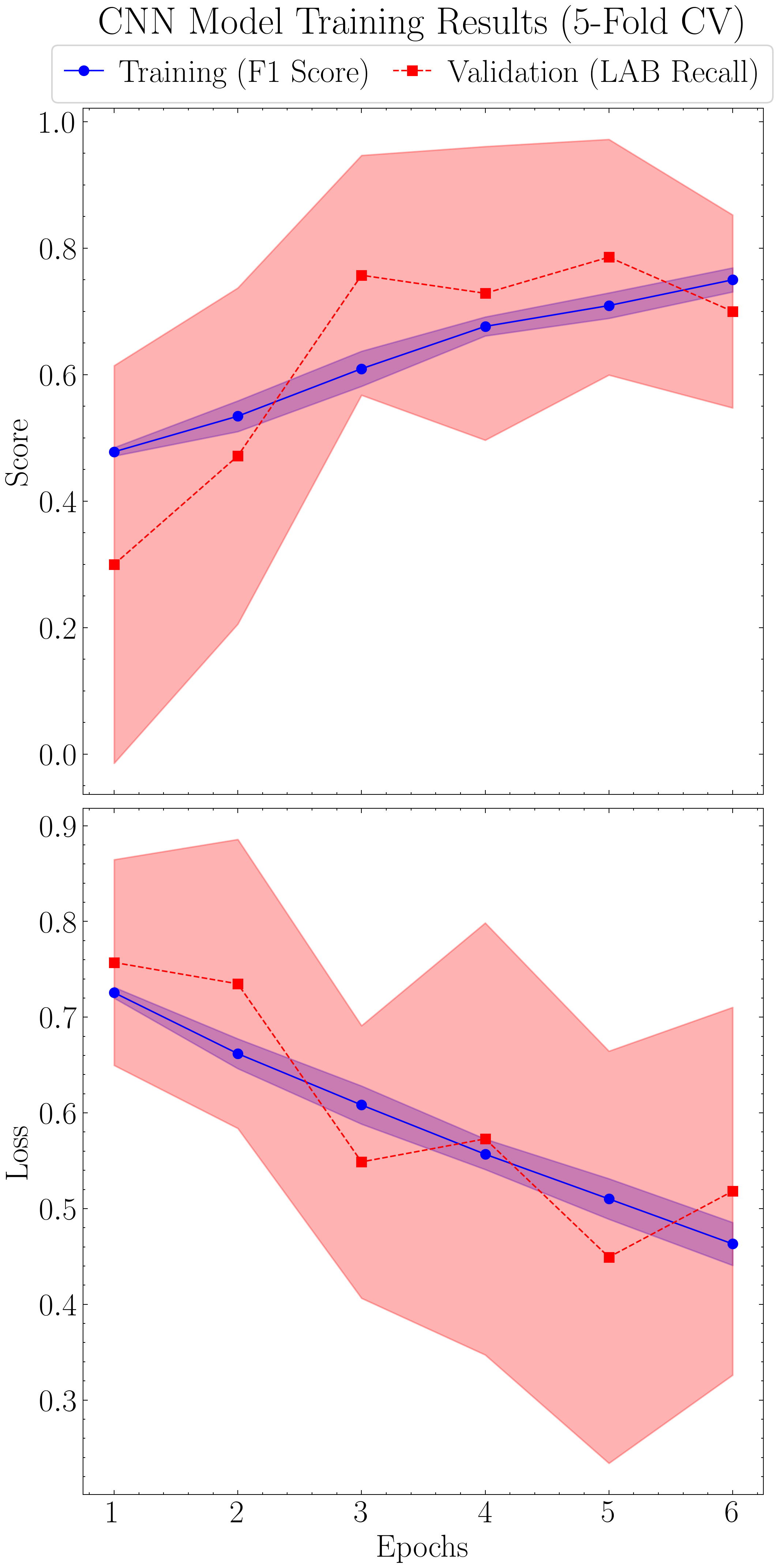
CNN Classification
We now classify the LAB training-set objects that passed our initial XGBoost classification step, along with the ~48,000 initial candidates identified as inliers by the iForest model. This CNN-filtered set is then saved for final analysis and prioritization.
import numpy as np
from pyBIA import cnn_model
from pyBIA.data_processing import concat_channels
from pyBIA.data_augmentation import resize

# Load the saved CNN model
model = cnn_model.Classifier()
model.load('cnn_model')

# Filter those with XGB probas greater than 0.9
priority_diffuse = np.load('priority_diffuse_final.npy')
priority_diffuse_names = np.loadtxt('priority_diffuse_names_final.txt', dtype=str)

# Need the difference image channel
bw_minus_r = priority_diffuse[:,:,:,0] / priority_diffuse[:,:,:,1]
bw_minus_r = np.expand_dims(bw_minus_r, axis=-1)
priority_diffuse = np.concatenate([priority_diffuse, bw_minus_r], axis=-1)

# Iterate through the five folds and classify only the training set instances that were in that validation fold
# Note that the built-in predict method handles this for us via the cv_model input (determines which model in the ensemble to use)
priority_diffuse_predictions = []
for i in range(5):
    sample = priority_diffuse[14*i:14*(i+1)]
    priority_diffuse_predictions.append(model.predict(sample, cv_model=i, return_proba=True))

priority_diffuse_predictions = np.vstack(priority_diffuse_predictions)
priority_diffuse_probas = priority_diffuse_predictions[:,1].astype('float')#[index]
order = np.argsort(priority_diffuse_probas)[::-1]

np.save('priority_diffuse_final_CNN_candidates.npy', priority_diffuse[order])
np.savetxt('priority_diffuse_final_CNN_candidates_names_probas.txt', np.c_[priority_diffuse_names[order], priority_diffuse_probas[order]], fmt='%s')

# Other diffuse candidates as selected by Prescott et al. 2012
# Note: These files include the singular non-detection hence need to remove it to avoid indexing issues later on!!!!

other_diffuse = np.load('other_diffuse_final.npy')
other_diffuse_names = np.loadtxt('other_diffuse_names_final.txt', dtype=str)

# Need the difference image channel
bw_minus_r = other_diffuse[:,:,:,0] / other_diffuse[:,:,:,1]
bw_minus_r = np.expand_dims(bw_minus_r, axis=-1)
other_diffuse = np.concatenate([other_diffuse, bw_minus_r], axis=-1)

# CNN prediction
other_diffuse_predictions = model.predict(other_diffuse, cv_model='all', return_proba=True)

#Save in order of highests to lowest probability predictions
other_diffuse_probas = other_diffuse_predictions[:,1].astype('float')#[index]
order = np.argsort(other_diffuse_probas)[::-1]
np.save('other_diffuse_final_CNN_candidates.npy', other_diffuse[order])
np.savetxt('other_diffuse_final_CNN_candidates_names_probas.txt', np.c_[other_diffuse_names[order], other_diffuse_probas[order]], fmt='%s')

# The initial candidates as selected by the XGBoost classifier

other_candidates_names = np.loadtxt('xgb_output_images_names.txt', dtype=str)
other_bw = np.load('xgb_output_images_bw.npy')
other_r = np.load('xgb_output_images_R.npy')

# Only need the inliers
iforest_preds = np.loadtxt('iforest_predictions.txt')
iforest_ypred = iforest_preds[:,0]
inlier_index = np.where(iforest_ypred == 1)[0]

# Resize and concat the images for classification, the predict method automatically resizes for us but here we do manually for faster processing
other_candidates_names = other_candidates_names[inlier_index]
other_bw = resize(other_bw[inlier_index], 70)
other_r = resize(other_r[inlier_index], 70)
other_candidates = concat_channels(other_bw, other_r)

# Need the difference image channel
bw_minus_r = other_candidates[:,:,:,0] / other_candidates[:,:,:,1]
bw_minus_r = np.expand_dims(bw_minus_r, axis=-1)
other_candidates = np.concatenate([other_candidates, bw_minus_r], axis=-1)

# CNN prediction
other_candidates_predictions = model.predict(other_candidates, cv_model='all', return_proba=True)

#Save in order of highests to lowest probas
other_candidate_probas = other_candidates_predictions[:,1].astype('float')#[index]
order = np.argsort(other_candidate_probas)[::-1]
np.save('OTHER_final_CNN_candidates.npy', other_candidates[order])
np.savetxt('OTHER_final_CNN_candidates_names_probas.txt', np.c_[other_candidates_names[order], other_candidate_probas[order]], fmt='%s')

## Now the five confirmed LABs
confirmed_diffuse_names = np.loadtxt('confirmed_diffuse_names.txt', dtype=str)
confirmed_diffuse = np.load('confirmed_diffuse.npy')

bw_minus_r = confirmed_diffuse[:,:,:,0] / confirmed_diffuse[:,:,:,1]
bw_minus_r = np.expand_dims(bw_minus_r, axis=-1)
confirmed_diffuse = np.concatenate([confirmed_diffuse, bw_minus_r], axis=-1)

# CNN prediction
confirmed_diffuse_predictions = model.predict(confirmed_diffuse, cv_model='all', return_proba=True)

np.savetxt('confirmed_candidates_final_CNN_names_probas.txt', np.c_[confirmed_diffuse_names, confirmed_diffuse_predictions[:,1]], fmt='%s')
These final candidate files can be downloaded below.
Images:
Corresponding names:
We can now visualize the probability-prediction distributions for both the LABs used to train the CNN (based on the five-fold CV results) and the ~48,000 initial candidates identified as inliers by the iForest model.
import numpy as np
import matplotlib.pyplot as plt
import pandas as pd
import scienceplots
plt.style.use('science')
plt.rcParams.update({'font.size': 21, 'lines.linewidth': 1.5})

# Load the CNN predictions on the initial candidates
candidates = np.loadtxt('OTHER_final_CNN_candidates_names_probas.txt', dtype=str)
candidates_names, candidates_cnn_probas = candidates[:,0], candidates[:,1].astype('float')

# The positive CNN training set data as per the validation results
lab_validation = np.loadtxt('priority_diffuse_final_CNN_candidates_names_probas.txt', dtype=str)
lab_validation_names, lab_validation_cnn_probas = lab_validation[:,0], lab_validation[:,1].astype('float')

n_bins = 8
bins = np.linspace(0, 1, n_bins + 1) # Common bin edges for both histograms

# Plot the histograms
fig, ax = plt.subplots(figsize=(8, 8))

ax.hist(candidates_cnn_probas, bins=bins,
        weights=np.ones_like(candidates_cnn_probas) / len(candidates_cnn_probas),
        histtype='step', color='blue', linewidth=1.5, linestyle='-',
        label='Initial Candidates')

ax.hist(lab_validation_cnn_probas, bins=bins,
        weights=np.ones_like(lab_validation_cnn_probas) / len(lab_validation_cnn_probas),
        histtype='step', color='green', linewidth=1.5, linestyle='--',
        label='Training LAB')

# Load the data for the confirmed LABs
confirmed_probas = np.loadtxt('confirmed_candidates_final_CNN_names_probas.txt', dtype=str)
confirmed_probas = confirmed_probas[:,1].astype('float')

# Confirmed LAB markers and colors
# Saved in the following order: 'PRG4, LABd05, PRG3, PRG2, PRG1'
special_items = {
    'LABd05': confirmed_probas[1],
    'PRG1': confirmed_probas[4],
    'PRG2': confirmed_probas[3],
    'PRG3': confirmed_probas[2],
    'PRG4': confirmed_probas[0]
}

special_colors = ['blue', 'green', 'cyan', 'purple', 'red']
special_markers = ['p', 'P', '>', "v", "^"]

# Add stars for the confirmed LABs
for (label, prob), color, marker in zip(special_items.items(), special_colors, special_markers):
    ax.scatter(prob, 0.0044, color=color, marker=marker, s=200, lw=3.5, alpha=0.9, label=label, edgecolor=color, facecolors='none')

ax.set_xlabel(r"$P\left(y = \mathrm{LAB} \mid \mathbf{X} \right)$")
ax.set_ylabel("Fraction of Objects")
ax.set_title('CNN Classification Results')
ax.legend(handletextpad=0.5, loc='upper left')

ax.axvline(0.6, linestyle=(0, (2, 2)), alpha=0.7, color='gray')
ax.annotate(r'Final Candidates $\downarrow$', xy=(0.64, 0.16), xytext=(-18, 0),
             textcoords='offset points', ha='right', va='bottom', color='gray', rotation=90)

plt.ylim((0,0.3))
plt.savefig('probability_hists.png', dpi=300, bbox_inches='tight')
plt.show()
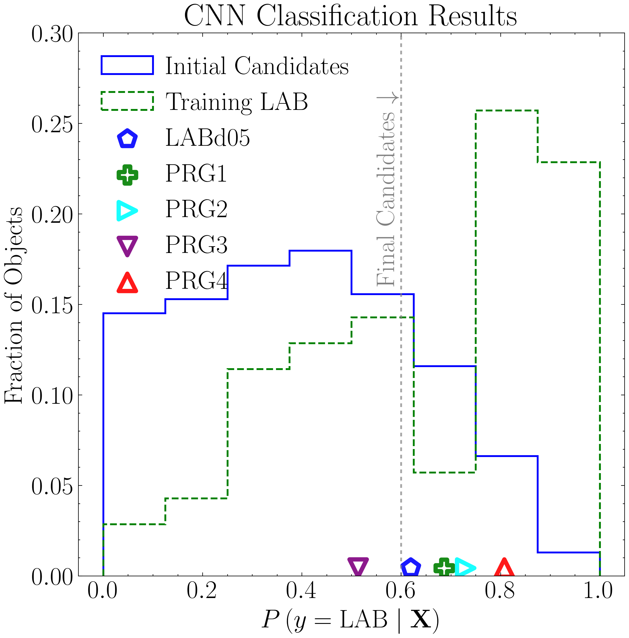
We now plot the binned averages of the probability predictions for the initial candidates as a function of the top three features used to train the XGBoost model.
import pandas as pd
import numpy as np
import matplotlib.pyplot as plt
import matplotlib as mpl
import scienceplots

plt.style.use('science')
plt.rcParams.update({'font.size': 21, 'lines.linewidth': 1.5})

error_mode = 'std' # Error bar options, we include 'std' or 'sem'
display_mode = 'quantiles' #  If std error mode can set this to 'errorbars' or 'shaded', otherwise 'quantiles'
pix_conversion = 3.8961 # NDWFS pix-to-arcsec
n_bins_other = 40 # No bins for histogram

# Data
priority_70 = np.loadtxt('priority_diffuse_final_CNN_candidates_names_probas.txt', dtype=str)
names_70 = priority_70[:, 0]
probas_70 = priority_70[:, 1].astype(float)

# Load the training data
# Where the training set files will be saved
nsig_path = 'nsigs/'

sig = 0.32 #Optimal sig from Fig. 2
df_diffuse_full = pd.read_csv(f'{nsig_path}_Bw_training_set_nsig_{sig}')

# Find the priority LABs we used to train the CNN
indices_70 = np.hstack([np.where(df_diffuse_full.obj_name == nm)[0] for nm in names_70])
df_diffuse = df_diffuse_full.iloc[indices_70].reset_index(drop=True)

# Load
all_xgb_probas = pd.read_csv("candidate_catalog_optimized_xgboost_8.csv")
candidates = np.loadtxt('OTHER_final_CNN_candidates_names_probas.txt', dtype=str)
candidates_names = candidates[:, 0]
candidates_cnn_probas = candidates[:, 1].astype(float)

# Compute indices to index the candidate catalog
indices_ = []
for _name_ in candidates_names:
    print('Computing indices...')
    index = np.where(all_xgb_probas.obj_name == _name_)[0]
    indices_.append(index[0])

# Hard-coding the probability prediction of the confirmed LABs
lab_info = {
    'NDWFS_J143410.9+331730': {'label': 'LABd05', 'cnn': 0.61917084},
    'NDWFS_J143512.2+351108': {'label': 'PRG1',  'cnn': 0.68620145},
    'NDWFS_J142623.0+351422': {'label': 'PRG2',  'cnn': 0.72969264},
    'NDWFS_J143412.7+332939': {'label': 'PRG3',  'cnn': 0.51314485},
    'NDWFS_J142653.1+343856': {'label': 'PRG4',  'cnn': 0.80759037}
}
special_colors  = ['blue', 'green', 'cyan', 'purple', 'red']
special_markers = ['p', 'P', '>', 'v', '^']

def get_feature_array(feature):
    # Return array for a feature over initial candidates, also logs lambda_1 and converts to arcsec
    if feature == 'mag':
        arr = np.array(all_xgb_probas.mag.iloc[indices_])
    elif feature == 'gini':
        arr = np.array(all_xgb_probas.gini.iloc[indices_])
    elif feature == 'covariance_eigval1':
        arr = np.array(all_xgb_probas.covariance_eigval1.iloc[indices_]) / (pix_conversion**2)
        arr = np.log10(arr)  # always log lambda1 (arcsec^2)
    else:
        raise ValueError("Unsupported feature")
    return arr

def get_feature_value_row(row, feature):
    # Return a single-row feature value (similar to above function but to be used by the single confirmed LAB instances)
    val = float(row[feature])
    if feature == 'covariance_eigval1':
        val = val / (pix_conversion**2)
        val = np.log10(val)  # always log lambda1 (arcsec^2)
    return val

def binned_stats(x, y, bins, error_mode='sem', display_mode='errorbars', pct1=25, pct2=75):
    # Compute binned centers and summary stats (median plus/minus error or quantiles)
    inds = np.digitize(x, bins)
    centers = (bins[:-1] + bins[1:]) / 2.0
    means, q25s, q75s, errors = [], [], [], []
    for i in range(1, len(bins)):
        mask = inds == i
        if np.any(mask):
            data_i = y[mask]
            means.append(np.percentile(data_i, 50))
            if display_mode == 'quantiles':
                q25s.append(np.percentile(data_i, pct1))
                q75s.append(np.percentile(data_i, pct2))
            else:
                err = np.std(data_i) / np.sqrt(np.sum(mask)) if error_mode == 'sem' else np.std(data_i)
                errors.append(err)
        else:
            means.append(np.nan)
            (q25s.append(np.nan), q75s.append(np.nan)) if display_mode == 'quantiles' else errors.append(np.nan)
    if display_mode == 'quantiles':
        return centers, np.array(means), np.array(q25s), np.array(q75s)
    return centers, np.array(means), np.array(errors)

def feature_title(feature):
    # Map feature key to a short LaTeX axis label
    if feature == 'mag': return r'$B_W$ Mag'
    if feature == 'gini': return r'Gini Index'
    if feature == 'covariance_eigval1': return r'$\log_{10}(\lambda_1)\ (\mathrm{arcsec}^2)$'
    return feature

def plot_feature_panel(ax, feature):
    # Plot feature vs. CNN probability with binned summary and annotations."""
    y_data = get_feature_array(feature)
    bins_other = np.linspace(0, 1, n_bins_other + 1)

    if display_mode == 'quantiles':
        centers, means, q25s, q75s = binned_stats(candidates_cnn_probas, y_data, bins_other, display_mode='quantiles')
        ax.plot(centers, means, color='black', label=r'Initial Candidates (n=47,829)')
        ax.fill_between(centers, q25s, q75s, color='gray', alpha=0.3)
    elif display_mode == 'errorbars':
        centers, means, errors = binned_stats(candidates_cnn_probas, y_data, bins_other, error_mode=error_mode, display_mode='errorbars')
        ax.errorbar(centers, means, yerr=errors, fmt='-', color='black', capsize=5, label=r'Initial Candidates (n=51,398)')
    else:
        centers, means, errors = binned_stats(candidates_cnn_probas, y_data, bins_other, error_mode=error_mode, display_mode='errorbars')
        ax.plot(centers, means, color='black', label=r'Initial Candidates (n=51,398)')
        ax.fill_between(centers, means - errors, means + errors, color='gray', alpha=0.3)

    for j in range(len(names_70)):
        fval = get_feature_value_row(df_diffuse.iloc[j], feature)
        lbl = "Training LAB (n=70)" if j == 0 else None
        ax.scatter(probas_70[j], fval, marker='o', s=200, facecolors='none', edgecolors='magenta',
                   linewidth=3.5, alpha=0.9, label=lbl)

    for i, (obj_name, info) in enumerate(lab_info.items()):
        lab_rows = df_diffuse_full[df_diffuse_full['obj_name'] == obj_name]
        if not lab_rows.empty:
            lab_val = get_feature_value_row(lab_rows.iloc[0], feature)
            ax.scatter(info['cnn'], lab_val, marker=special_markers[i], s=200,
                       facecolors='none', edgecolors=special_colors[i],
                       linewidth=3.5, alpha=0.9, label=info['label'])

    ax.set_ylabel(feature_title(feature))
    if feature == 'mag':
        ax.set_ylim((22.4, 24.2))
        ax.invert_yaxis()

    handles, labels = ax.get_legend_handles_labels()
    uniq = dict(zip(labels, handles))
    ax.legend([], [])
    return uniq

features = ['mag', 'gini', 'covariance_eigval1']

fig, (ax1, ax2, ax3) = plt.subplots(1, 3, figsize=(24, 8), sharey=False)
fig.subplots_adjust(top=0.85, wspace=0.15)

uniq1 = plot_feature_panel(ax1, features[0])
plot_feature_panel(ax2, features[1])
plot_feature_panel(ax3, features[2])

ax2.set_title('CNN Model Performance Analysis', y=1.1)
for ax in (ax1, ax2, ax3):
    ax.set_xlabel(r"$P\left(y = \mathrm{LAB} \mid \mathbf{X} \right)$")

handles1, labels1 = [], []
for lbl, h in uniq1.items():
    if lbl is not None:
        labels1.append(lbl)
        handles1.append(h)

fig.legend(handles1, labels1, loc='upper center', bbox_to_anchor=(0.5, 0.94), ncol=7,
           frameon=True, fancybox=True, handlelength=1)

plt.savefig('three_panel_feature_vs_prob_columns.png', dpi=300, bbox_inches='tight')
plt.show()
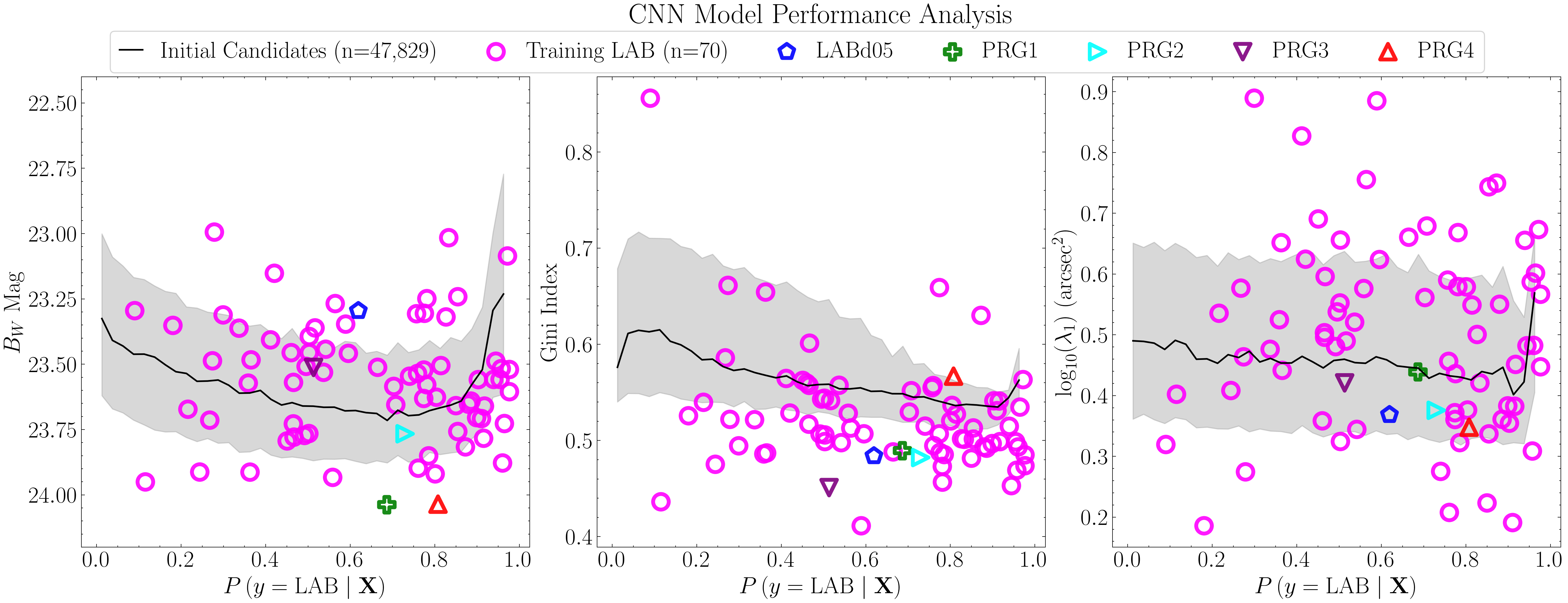
Candidate Prioritization
We now prioritize the final candidates for spectroscopic follow-up based on their similarity to the known LABs.
Priority candidates are selected according to their Bw area, Bw–R color, and Bw-based Gini index. To perform the color selection, we first compute the R-band magnitudes using the Catalog class.
import numpy as np
import pandas as pd
from pyBIA import catalog
from astropy.io import fits

# Load the original XGB candidate catalog (~234k objects)
csv_candidates = pd.read_csv('candidate_catalog_optimized_xgboost_8.csv')

# Load the names and probabilities of the candidates that were positively classified by the CNN
candidate_names_probas = np.loadtxt('OTHER_final_CNN_candidates_names_probas.txt', dtype=str)
index = np.where(candidate_names_probas[:,1].astype('float') >= 0.5)[0]
candidate_names_probas = candidate_names_probas[index]

# Index the csv to only these positive candidates
candidates_indices = []
for i in range(len(csv_candidates)):
    if csv_candidates.obj_name.iloc[i] in candidate_names_probas[:,0]:
        candidates_indices.append(i)

csv_candidates = csv_candidates.iloc[candidates_indices]

# Load the diffuse training objects
# Where the training set files will be saved
nsig_path = 'nsigs/'
sig = 0.32 #Optimal sig from Fig. 2
training_set = pd.read_csv(f'{nsig_path}_Bw_training_set_nsig_{sig}')

blob_index = np.where(training_set['flag'] == 1)[0] # Select only the diffuse objects
training_set = training_set.iloc[blob_index]

# Will load the names of the five confirmed blobs to create a subsample dataframe, will be used for color-color selection
confirmed_diffuse_names = np.loadtxt('confirmed_LAB_names.txt', dtype=str)

confirmed_diffuse_indices = []
for i in range(len(training_set)):
    if training_set.obj_name.iloc[i] in confirmed_diffuse_names:
        confirmed_diffuse_indices.append(i)

confirmed_set = training_set.iloc[confirmed_diffuse_indices]

# Now load the names of the diffuse training objects selected by the CNN, not including the confirmed blobs
priority_diffuse_names_probas = np.loadtxt('priority_diffuse_final_CNN_candidates_names_probas.txt', dtype=str)
index = np.where(priority_diffuse_names_probas[:,1].astype('float') >= 0.5)[0]
priority_diffuse_names_probas = priority_diffuse_names_probas[index]

other_diffuse_names_probas = np.loadtxt('other_diffuse_final_CNN_candidates_names_probas.txt', dtype=str)
index = np.where(other_diffuse_names_probas[:,1].astype('float') >= 0.5)[0]
other_diffuse_names_probas = other_diffuse_names_probas[index]

diffuse_indices = []
for i in range(len(training_set)):
    if training_set.obj_name.iloc[i] in np.r_[priority_diffuse_names_probas[:,0], other_diffuse_names_probas[:,0]]:
        diffuse_indices.append(i)

training_set = training_set.iloc[diffuse_indices]

# Combine the two dataframes, this is the Bw band, doesn't include the five confirmed
final_candidate_catalog_bw = pd.concat([csv_candidates, training_set], ignore_index=True)
final_candidate_catalog_bw.to_csv('_Bw_FINAL_candidate_catalog.csv', chunksize=1000)

# Save a dataframe with only the confirmed blobs, to be used for the color-color selection below
confirmed_set.to_csv('_Bw_FINAL_confirmed_catalog.csv')

# Create a new catalog in the R band for the final candidates (see above, includes both new others and original training set)

data_path = 'NDWFS/fits_images/R_FITS/'
data_error_path = 'NDWFS/fits_images/rms_images/R/npy/'

frame = [] #To store all 27 subfields
for fieldname in np.unique(np.array(final_candidate_catalog_bw['field_name'])):

    print(fieldname)

    # Load the field data
    data_hdu, error_map = fits.open(data_path+fieldname+'_R_03_reg_fix.fits'), np.load(data_error_path+fieldname+'_R_03_rms.npy')

    # Extract the data and corresponding ZP
    data_map, zeropoint, exptime = data_hdu[0].data, data_hdu[0].header['MAGZERO'], data_hdu[0].header['EXPTIME']

    # Select only the samples from this subfield
    subfield_index = np.where(final_candidate_catalog_bw['field_name']==fieldname)[0]
    xpix, ypix = final_candidate_catalog_bw[['xpix', 'ypix']].iloc[subfield_index].values.T
    objname, field, flag = final_candidate_catalog_bw[['obj_name', 'field_name', 'flag']].iloc[subfield_index].values.T

    # Create the catalog object
    cat = catalog.Catalog(data_map, error=error_map, x=xpix, y=ypix, zp=zeropoint, exptime=exptime, nsig=sig, flag=flag, obj_name=objname, field_name=field, invert=True)

    # Generate the catalog and append the ``cat`` attribute to the frame list
    cat.create(save_file=False); frame.append(cat.cat)

# Combine all 27 sub-catalogs into one master frame and save
frame = pd.concat(frame, axis=0, join='inner'); frame.to_csv('_R_FINAL_candidate_catalog.csv', chunksize=1000)

# Create a new catalog in the R band for the five confirmed blobs
data_path = 'NDWFS/fits_images/R_FITS/'
data_error_path = 'NDWFS/fits_images/rms_images/R/npy/'

frame = [] #To store all 27 subfields
for fieldname in np.unique(np.array(confirmed_set['field_name'])):

    # Load the field data
    data_hdu, error_map = fits.open(data_path+fieldname+'_R_03_reg_fix.fits'), np.load(data_error_path+fieldname+'_R_03_rms.npy')

    # Extract the data and corresponding ZP and exposure time
    data_map, zeropoint, exptime = data_hdu[0].data, data_hdu[0].header['MAGZERO'], data_hdu[0].header['EXPTIME']

    # Select only the samples from this subfield
    subfield_index = np.where(confirmed_set['field_name']==fieldname)[0]
    xpix, ypix = confirmed_set[['xpix', 'ypix']].iloc[subfield_index].values.T
    objname, field, flag = confirmed_set[['obj_name', 'field_name', 'flag']].iloc[subfield_index].values.T

    # Create the catalog object
    cat = catalog.Catalog(data_map, error=error_map, x=xpix, y=ypix, zp=zeropoint, exptime=exptime, nsig=sig, flag=flag, obj_name=objname, field_name=field, invert=True)

    # Generate the catalog and append the ``cat`` attribute to the frame list
    cat.create(save_file=False); frame.append(cat.cat)

# Combine all 27 sub-catalogs into one master frame and save
frame = pd.concat(frame, axis=0, join='inner'); frame.to_csv('_R_FINAL_confirmed_catalog.csv')
We can now generate the plot, applying a top-down filtering approach to select the prioritized candidates.
import numpy as np
import pandas as pd
import matplotlib.pyplot as plt
from matplotlib.lines import Line2D
import scienceplots

plt.style.use("science")
plt.rcParams.update({"font.size": 21, "lines.linewidth": 1.5})

pix_conversion = 3.8961  # NDWFS survey pixel-per-arcsecond

# Load the final candidates and confirmed catalogs we generated for both Bw and R bands
final_candidate_catalog_bw = pd.read_csv('_Bw_FINAL_candidate_catalog.csv').sort_values('obj_name').reset_index(drop=True)
final_candidate_catalog_r = pd.read_csv('_R_FINAL_candidate_catalog.csv').sort_values('obj_name').reset_index(drop=True)

final_confirmed_catalog_bw = pd.read_csv('_Bw_FINAL_confirmed_catalog.csv').sort_values('obj_name').reset_index(drop=True)
final_confirmed_catalog_r = pd.read_csv('_R_FINAL_confirmed_catalog.csv').sort_values('obj_name').reset_index(drop=True)

confirmed_color_diff = final_confirmed_catalog_bw.mag - final_confirmed_catalog_r.mag
final_candidate_color_diff = final_candidate_catalog_bw.mag - final_candidate_catalog_r.mag

# Set the Bw-R color and Bw-based area selection thresholds
color_thresh, area_thresh, upper_area_thresh = 0.8, 850, 2000
idx_priority = np.where((final_candidate_color_diff <= color_thresh) &
                        (final_candidate_catalog_bw.area >= area_thresh) &
                        (final_candidate_catalog_bw.area <= upper_area_thresh))[0]

idx_non_priority = [i for i in range(len(final_candidate_color_diff)) if i not in idx_priority]

# Load the CNN probability predictions
other_names = np.loadtxt('OTHER_final_CNN_candidates_names_probas.txt', dtype=str)
diffuse_other = np.loadtxt('other_diffuse_final_CNN_candidates_names_probas.txt', dtype=str)
diffuse_priority = np.loadtxt('priority_diffuse_final_CNN_candidates_names_probas.txt', dtype=str)

candidate_names = np.r_[other_names[:, 0], diffuse_other[:, 0], diffuse_priority[:, 0]]
candidate_probas = np.r_[other_names[:, 1], diffuse_other[:, 1], diffuse_priority[:, 1]].astype(float)

# Need to reorder probas to match the order as they appear in the Bw-based catalog
order_idx = [np.where(candidate_names == n)[0][0] for n in final_candidate_catalog_bw.obj_name]
candidate_probas = candidate_probas[order_idx]

#  Create the full arrays
def subset(catalog, idx): return catalog.iloc[idx]

Final_Candidates_Color = subset(final_candidate_color_diff, idx_priority)
Final_Candidates_Area = subset(final_candidate_catalog_bw.area, idx_priority)
Final_Candidates_Gini = subset(final_candidate_catalog_bw.gini, idx_priority)
Final_Candidates_Probas = candidate_probas[idx_priority]

Final_Candidates_Color_N = subset(final_candidate_color_diff, idx_non_priority)
Final_Candidates_Area_N = subset(final_candidate_catalog_bw.area, idx_non_priority)
Final_Candidates_Gini_N = subset(final_candidate_catalog_bw.gini, idx_non_priority)
Final_Candidates_Probas_N = candidate_probas[idx_non_priority]

ALL_COLOR_0 = np.r_[Final_Candidates_Color, Final_Candidates_Color_N]
ALL_AREA_0 = np.r_[Final_Candidates_Area, Final_Candidates_Area_N]
ALL_GINI_0 = np.r_[Final_Candidates_Gini, Final_Candidates_Gini_N]
ALL_PROBAS_0 = np.r_[Final_Candidates_Probas, Final_Candidates_Probas_N]

#  The five confirmed LABs
conf_names = np.loadtxt('confirmed_candidates_final_CNN_names_probas.txt', dtype=str,  usecols=0)
conf_probas = np.loadtxt('confirmed_candidates_final_CNN_names_probas.txt', dtype=float, usecols=1)
conf_idx = [np.where(conf_names == n)[0][0] for n in final_confirmed_catalog_bw.obj_name]

Confirmed_Color = confirmed_color_diff.iloc[::-1]
Confirmed_Area = final_confirmed_catalog_bw.area.iloc[::-1]
Confirmed_Gini = final_confirmed_catalog_bw.gini.iloc[::-1]
Confirmed_Probas = conf_probas[conf_idx][::-1]
names_lab = ['PRG2', 'PRG4', 'LABd05', 'PRG3', 'PRG1'][::-1]

special_colors  = ['cyan', 'red', 'blue', 'purple', 'green'][::-1]
special_markers = ['>', '^', 'p', 'v', 'P'][::-1]

def finite_pair(x, y):
    # Return x,y filtered to finite pairs only (i.e., no NaN/Inf)
    x = np.asarray(x, dtype=float)
    y = np.asarray(y, dtype=float)
    m = np.isfinite(x) & np.isfinite(y)
    return x[m], y[m]

def sanitize_1d(arr):
    # Filter a single array to finite values only
    arr = np.asarray(arr, dtype=float)
    return arr[np.isfinite(arr)]

# Function to plot the panels
def plot_histogram_with_avg_proba_axes(
        ax1, x, probas, xlabel, ylabel_hist, ylabel_avg, *,
        bins=12, xlim=None, ylim=None,
        vline_vals=None, arrow_dirs=None,
        shaded_regions=None,
        confirmed_points=None, confirmed_marker_colors=None,
        confirmed_names=None, confirmed_marker_style=None,
        confirmed_points_ymin=0.004):

    x, probas = finite_pair(x, probas)
    if x.size == 0:
        raise ValueError(f"No finite data to plot for {xlabel}")

    # histogram (fraction of objects)
    weights = np.ones_like(x) / len(x)
    n, edges, _ = ax1.hist(x, bins=bins, weights=weights, histtype='step',
                           color='b', alpha=0.6, label='Initial Candidates')
    ax1.set_xlabel(xlabel)
    ax1.set_ylabel(ylabel_hist)
    if xlim: ax1.set_xlim(xlim)
    if ylim: ax1.set_ylim(ylim)

    # shaded regions
    if shaded_regions:
        for x0, x1 in shaded_regions:
            ax1.axvspan(x0, x1, color='gray', alpha=0.25, zorder=-5)

    # probability curve + std-dev band
    centers = (edges[:-1] + edges[1:]) / 2
    means = []
    stds  = []
    for i in range(len(edges) - 1):
        mask = (x >= edges[i]) & (x < edges[i+1] if i < len(edges)-2 else x <= edges[i+1])
        if np.any(mask):
            means.append(np.mean(probas[mask]))
            stds.append(np.std (probas[mask]))
        else:
            means.append(np.nan)
            stds.append(np.nan)

    ax2 = ax1.twinx()
    ax2.plot(centers, means, color='red', label=r'$\langle P(y=\mathrm{LAB}\mid\mathbf{X}) \rangle$')
    ax2.fill_between(centers, np.array(means)-np.array(stds),
                     np.array(means)+np.array(stds),
                     color='red', alpha=0.30)
    ax2.set_ylabel(ylabel_avg)

    # confirmed LAB markers along the baseline
    if confirmed_points is not None:
        confirmed_points = sanitize_1d(confirmed_points)
        if confirmed_marker_colors is None or confirmed_marker_style is None or confirmed_names is None:
            pass  # nothing to draw
        else:
            n_confirmed = min(len(confirmed_points), len(confirmed_marker_colors), len(confirmed_marker_style), len(confirmed_names))
            for pt, col, mk, nm in zip(confirmed_points[:n_confirmed],
                                       confirmed_marker_colors[:n_confirmed],
                                       confirmed_marker_style[:n_confirmed],
                                       confirmed_names[:n_confirmed]):
                if np.isfinite(pt):
                    ax1.scatter(pt, confirmed_points_ymin, marker=mk, s=400,
                                facecolors='none', edgecolors=col, linewidth=3.5, label=nm)

    # green v-lines + arrows
    if vline_vals:
        arrow_dirs = arrow_dirs or ['left'] * len(vline_vals)
        x_min, x_max = ax1.get_xlim()
        offset = 0.1 * (x_max - x_min)
        y_min, y_max = ax1.get_ylim()
        y_arrow = y_min + 0.98 * (y_max - y_min)
        for v, direction in zip(vline_vals, arrow_dirs):
            if np.isfinite(v):
                ax1.axvline(v, color='green', linestyle='--')
                if direction == 'left':
                    ax1.annotate('', xy=(v, y_arrow), xytext=(v + offset, y_arrow),
                                 arrowprops=dict(arrowstyle="->", color='green'))
                else:
                    ax1.annotate('', xy=(v, y_arrow), xytext=(v - offset, y_arrow),
                                 arrowprops=dict(arrowstyle="->", color='green'))


# Do the prioritization, first those that made it through the CNN with proba >= 0.6, then the area, color and Gini
# FILTER 1 — PROBA ≥ 0.6
sel1 = (ALL_PROBAS_0 >= 0.6)
ALL_COLOR_1 = ALL_COLOR_0[sel1]
ALL_AREA_1 = ALL_AREA_0[sel1]
ALL_GINI_1 = ALL_GINI_0[sel1]
ALL_PROBAS_1 = ALL_PROBAS_0[sel1]

# FILTER 2 — AREA BETWEEN THRESHOLDS
sel2 = (ALL_AREA_1 >= area_thresh) & (ALL_AREA_1 <= upper_area_thresh)
ALL_COLOR_2 = ALL_COLOR_1[sel2]
ALL_AREA_2 = ALL_AREA_1[sel2]
ALL_GINI_2 = ALL_GINI_1[sel2]
ALL_PROBAS_2 = ALL_PROBAS_1[sel2]

# FILTER 3 — COLOR <= THRESHOLD
sel3 = np.isfinite(ALL_COLOR_2) & (ALL_COLOR_2 <= color_thresh)
ALL_COLOR_3 = ALL_COLOR_2[sel3]
ALL_AREA_3 = ALL_AREA_2[sel3]
ALL_GINI_3 = ALL_GINI_2[sel3]
ALL_PROBAS_3 = ALL_PROBAS_2[sel3]

# Plot
fig, (ax_area, ax_color, ax_gini) = plt.subplots(3, 1, figsize=(8, 24), sharex=False)
fig.subplots_adjust(top=0.9, hspace=0.15)

# PANEL 1 — AREA
area_low  = area_thresh / pix_conversion**2
area_high = upper_area_thresh / pix_conversion**2
plot_histogram_with_avg_proba_axes(
    ax_area,
    ALL_AREA_1 / pix_conversion**2, ALL_PROBAS_1,
    xlabel=r"$B_W$ Area ($\rm arcsec^2$)",
    ylabel_hist=f"Fraction of Objects (n={len(ALL_AREA_1):,})",
    ylabel_avg='CNN Probability Prediction',
    bins=25, xlim=(0, 460),
    vline_vals=[area_low, area_high],
    arrow_dirs=["right", "left"],
    shaded_regions=[(0, area_low), (area_high, 460)],
    confirmed_points=Confirmed_Area / pix_conversion**2,
    confirmed_marker_colors=special_colors,
    confirmed_names=names_lab,
    confirmed_marker_style=special_markers,
    confirmed_points_ymin=0.0056
    )

# PANEL 2 — COLOR
plot_histogram_with_avg_proba_axes(
    ax_color,
    ALL_COLOR_2, ALL_PROBAS_2,
    xlabel=r"$B_W - R$",
    ylabel_hist=f"Fraction of Objects (n={len(ALL_COLOR_2):,})",
    ylabel_avg='CNN Probability Prediction',
    bins=25, xlim=(-3, 3.4),
    vline_vals=[color_thresh],
    arrow_dirs=["left"],
    shaded_regions=[(color_thresh, 3.4)],
    confirmed_points=Confirmed_Color,
    confirmed_marker_colors=special_colors,
    confirmed_names=names_lab,
    confirmed_marker_style=special_markers,
    confirmed_points_ymin=0.0102
    )

# PANEL 3 — GINI
gini_cut = 0.49
plot_histogram_with_avg_proba_axes(
    ax_gini,
    ALL_GINI_3, ALL_PROBAS_3,
    xlabel="Gini Index",
    ylabel_hist = f"Fraction of Objects (n={len(ALL_GINI_3):,})",
    ylabel_avg='CNN Probability Prediction',
    bins=25, xlim=(0.35, 0.95),
    vline_vals=[gini_cut],
    arrow_dirs=["left"],
    shaded_regions=[(gini_cut, 1.0)],
    confirmed_points=Confirmed_Gini,
    confirmed_marker_colors=special_colors,
    confirmed_names=names_lab,
    confirmed_marker_style=special_markers,
    confirmed_points_ymin=0.005
    )

# Top title
ax_area.set_title('Priority Candidate Selection', y=1.18)

# Legend in order for aesthetics
legend_elements = [
    Line2D([0],[0], color='b', lw=1.5, label='Initial Candidates'),
    Line2D([0],[0], color='red', lw=1.5, label=r'$\langle P(y=\mathrm{LAB}\mid\mathbf{X}) \rangle$'),
    Line2D([0],[0], marker='p', markersize=16, markerfacecolor='none',
           markeredgewidth=3.5, markeredgecolor='blue', linestyle='None', label='LABd05'),
    Line2D([0],[0], marker='v', markersize=16, markerfacecolor='none',
           markeredgewidth=3.5, markeredgecolor='purple', linestyle='None', label='PRG3'),
    Line2D([0],[0], marker='P', markersize=16, markerfacecolor='none',
           markeredgewidth=3.5, markeredgecolor='green', linestyle='None', label='PRG1'),
    Line2D([0],[0], marker='^', markersize=16, markerfacecolor='none',
           markeredgewidth=3.5, markeredgecolor='red', linestyle='None', label='PRG4'),
    Line2D([0],[0], marker='>', markersize=16, markerfacecolor='none',
           markeredgewidth=3.5, markeredgecolor='cyan', linestyle='None', label='PRG2'),
]

fig.legend(legend_elements,
           [h.get_label() for h in legend_elements],
           loc='upper center', bbox_to_anchor=(0.5, 0.947), ncol=4,
           frameon=True, fancybox=True, handlelength=0.9,
           columnspacing=0.9, handletextpad=0.5)

plt.savefig('priority_selection_three_panel.png', dpi=300, bbox_inches='tight')
plt.show()
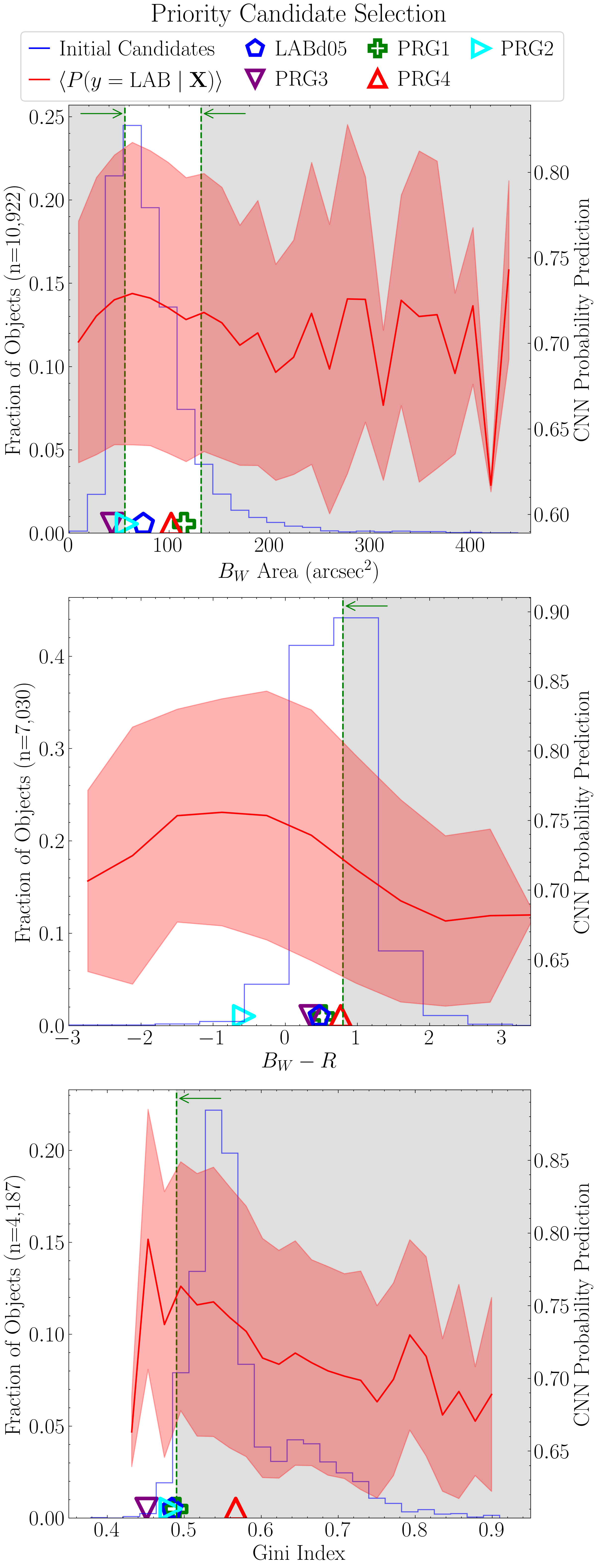
Final Catalogs and Candidates
We can now compile a complete catalog of all the sources in NDWFS Boötes, incorporating both the iForest and CNN probability scores. Because the catalogs used thus far have omitted RA and DEC, this code produces a final comprehensive catalog containing all scores and segmentation-based features, after which we append the RA and DEC positions from the following file: ndwfs_bootes_extracted_from_DW.
import numpy as np
import pandas as pd
from pyBIA import data_processing

candidate_catalog = pd.read_csv('candidate_catalog_optimized_xgboost_8.csv')
non_candidate_catalog = pd.read_csv('non_candidate_catalog_xgboost_8.csv')

# Remember the OTHER were already included in the above catalogs according to the LoO
# Where the training set files will be saved
nsig_path = 'nsigs/'

sig = 0.32 #Optimal sig from Fig. 2

training_set = pd.read_csv(f'{nsig_path}_Bw_training_set_nsig_{sig}')
index = np.where(training_set.flag == 1)[0]
training_set = training_set.iloc[index]

loo_lab = np.loadtxt('LoO_LAB', dtype=str)
lab_names = loo_lab[:,0]
lab_probas = loo_lab[:,2].astype('float')

loo_confirmed = np.loadtxt('LoO_Confirmed_LAB', dtype=str)
confirmed_names = ['NDWFS_J143410.9+331730', 'NDWFS_J143512.2+351108', 'NDWFS_J142623.0+351422', 'NDWFS_J143412.7+332939', 'NDWFS_J142653.1+343856'] #loo_confirmed[:,0]
confirmed_probas = loo_confirmed[:,2].astype('float')

all_lab_names = np.r_[lab_names, confirmed_names]
all_lab_probas = np.r_[lab_probas, confirmed_probas]

training_set['proba'] = np.zeros(len(training_set))
for i in range(len(training_set)):
        index = np.where(all_lab_names == training_set.obj_name.iloc[i])[0]
        training_set['proba'].iloc[i] = all_lab_probas[index] if len(index) == 1 else np.nan

# To make a master catalog first revert the non_candidate_catalog probabilities since these are the probas of not being LAB
non_candidate_catalog.proba = 1 - non_candidate_catalog.proba

# Now all three catalogs have an appropriate proba column
combined_df = pd.concat([training_set, candidate_catalog, non_candidate_catalog])
combined_df = combined_df.drop(['Unnamed: 0.1', 'Unnamed: 0'], axis=1)

hu_cols = ['Hu1', 'Hu2', 'Hu3', 'Hu4', 'Hu5', 'Hu6', 'Hu7']

# The above combined_df does not contain the non-detections (except for the single LAB training class LAB)
original_master = pd.read_csv('Other_Catalog_Master_0.32')

non_detections = np.where((original_master.area == -999) | (~np.isfinite(original_master.mag)) | (~np.isfinite(original_master[hu_cols]).all(axis=1)))[0]
original_master = original_master.iloc[non_detections]
original_master['proba'] = [np.nan] * len(original_master)

final_master = pd.concat([combined_df, original_master])
final_master = final_master.drop(['Unnamed: 0'], axis=1)
final_master.rename(columns={'proba': 'XGBoost8_Proba'}, inplace=True)

# Now add the outlier scores (NOTE THAT THE LAB CLASS DOES NOT HAVE OUTLIER SCORES SINCE THESE WERE USED TO TRAIN THE IFOREST!)
iforest_results = np.loadtxt('outlier_scores_and_areas.txt', dtype=str)
iforest_names = iforest_results[:,0]
iforest_scores = iforest_results[:,2].astype('float')

final_master['iForest_scores'] = [np.nan] * len(final_master)

for i in range(len(iforest_names)):
        index = np.where(final_master.obj_name == iforest_names[i])[0]
        final_master['iForest_scores'].iloc[index] = iforest_scores[i] if len(index) == 1 else np.nan

# Now the CNN probas
other_cnn = np.loadtxt('OTHER_final_CNN_candidates_names_probas.txt', dtype=str)
lab_cnn = np.loadtxt('other_diffuse_final_CNN_candidates_names_probas.txt', dtype=str)
lab_priority_cnn = np.loadtxt('priority_diffuse_final_CNN_candidates_names_probas.txt', dtype=str)
lab_confirmed_cnn = np.loadtxt('confirmed_candidates_final_CNN_names_probas.txt', dtype=str)

all_names = np.r_[other_cnn[:,0], lab_cnn[:,0], lab_priority_cnn[:,0], lab_confirmed_cnn[:,0]]
all_cnn_probas = np.r_[other_cnn[:,1], lab_cnn[:,1], lab_priority_cnn[:,1], lab_confirmed_cnn[:,1]]
all_cnn_probas = all_cnn_probas.astype('float')

final_master['CNN_proba'] = [np.nan] * len(final_master)
for i in range(len(all_names)):
        index = np.where(final_master.obj_name == all_names[i])[0]
        final_master['CNN_proba'].iloc[index] = all_cnn_probas[i] if len(index) == 1 else np.nan

# Now add the color
final_candidate_catalog_bw = pd.read_csv('_Bw_FINAL_candidate_catalog.csv').sort_values('obj_name').reset_index(drop=True)
final_candidate_catalog_r = pd.read_csv('_R_FINAL_candidate_catalog.csv').sort_values('obj_name').reset_index(drop=True)

final_confirmed_catalog_bw = pd.read_csv('_Bw_FINAL_confirmed_catalog.csv').sort_values('obj_name').reset_index(drop=True)
final_confirmed_catalog_r = pd.read_csv('_R_FINAL_confirmed_catalog.csv').sort_values('obj_name').reset_index(drop=True)

confirmed_color_diff = final_confirmed_catalog_bw.mag - final_confirmed_catalog_r.mag
final_candidate_color_diff = final_candidate_catalog_bw.mag - final_candidate_catalog_r.mag

final_master['Color'] = [np.nan] * len(final_master)

for i in range(len(final_confirmed_catalog_bw)):
        index = np.where(final_master.obj_name == final_confirmed_catalog_bw.obj_name.iloc[i])[0]
        final_master['Color'].iloc[index] = confirmed_color_diff.iloc[i] if len(index) == 1 else np.nan

for i in range(len(final_candidate_catalog_bw)):
        index = np.where(final_master.obj_name == final_candidate_catalog_bw.obj_name.iloc[i])[0]
        final_master['Color'].iloc[index] = final_candidate_color_diff.iloc[i] if len(index) == 1 else np.nan

# Finally save the ra and dec which up until now have been stored here
survey_objects = pd.read_csv('ndwfs_bootes_extracted_from_DW')

final_master['ra'] = np.zeros(len(final_master))
final_master['dec'] = np.zeros(len(final_master))

ra, dec = [], []
for i in range(len(final_master)):
        index = np.where((survey_objects.NDWFS_objname == final_master.obj_name.iloc[i]) & (survey_objects.field_name == final_master.field_name.iloc[i]))[0]
        if len(index) >= 2: # If there are duplicates (e.g., objects near edge of subfield that falls in multiple subfields)
                index = index[0]
        ra.append(float(survey_objects.ra.iloc[index]))
        dec.append(float(survey_objects.dec.iloc[index]))

# Now set the columns
final_master['ra'] = ra
final_master['dec'] = dec

#Finally save this master cat which contains 2,377,342 (from the Table in paper) plus the 860 LAB candidates we train with
final_master.to_csv('final_master_catalog.csv')
This final master catalog containing all sources, features, and scores, is available for download here.
This catalog includes every source in NDWFS Boötes, including non-detections and duplicate objects (i.e., those located close together and effectively representing the same system as seen by our models). We now generate a sub-catalog of only the priority candidates identified in earlier stages and remove any duplicates. Duplicate objects are flagged if they lie within 10 arcseconds of one another, in which case only one is retained. This step is essential because the group-like nature of LABs often results in multiple galaxies being cataloged as distinct sources by NDWFS but, for our purposes, should be treated as a single object. After removing duplicates, we perform a final visual inspection to remove any remaining outlier sources that may still be present.
import pandas as pd
import numpy as np
from astropy.coordinates import SkyCoord
import astropy.units as u
from pyBIA.data_processing import concat_channels

# Load the master cat
final_master = pd.read_csv('final_master_catalog.csv')

# Our priority candidate selection
priority_index = np.where((final_master.XGBoost8_Proba >= 0.9) & (final_master.CNN_proba >= 0.6) & (final_master.area >= 850) & (final_master.area <= 2000) & (final_master.Color <= 0.8) & (np.isfinite(final_master.Color)) & (final_master.gini <= 0.49))[0]
priority_cat = final_master.iloc[priority_index]

# Function to identify the duplicate objects
def dedupe_by_angular_separation(
    df: pd.DataFrame,
    ra_col: str = "ra", # As the column shows in the dataframe
    dec_col: str = "dec", # As the column shows in the dataframe
    sep_arcsec: float = 10.0, # Arcsec separation to consider duplicates
    keep: str = "first", # "first", "max", or "min"
    score_col: str | None = None): # Only used if keep is either "max" or "min", to determine which source to keep among the group
    #Remove duplicate rows from a DataFrame based on angular separation of sky coordinates, keeping only one per group and returning the cleaned DataFrame plus a table of grouped duplicates.

    # Work on a reset-index
    work = df.reset_index().rename(columns={"index": "orig_idx"}).copy()

    # Build coordinates and find all pairs within sep_arcsec
    coords = SkyCoord(ra=work[ra_col].values * u.deg, dec=work[dec_col].values * u.deg, frame="icrs")
    i1, i2, sep, _ = coords.search_around_sky(coords, sep_arcsec * u.arcsec)

    # Keep only (i<j) to avoid self-pairs and double counting
    m = i1 < i2
    pairs = np.column_stack([i1[m], i2[m]])
    if pairs.size == 0:
        # No duplicates found
        groups = pd.DataFrame(columns=["group_id","kept","orig_idx","ra","dec","sep_to_keep_arcsec"])
        return df.copy(), groups

    # Do a union-find to get the components
    parent = np.arange(len(work))

    def find(x):
        while parent[x] != x:
            parent[x] = parent[parent[x]]
            x = parent[x]
        return x

    def union(a, b):
        ra, rb = find(a), find(b)
        if ra != rb:
            parent[rb] = ra

    for a, b in pairs:
        union(a, b)

    # Interate and collect members per
    comp = {}
    for idx in range(len(work)):
        root = find(idx)
        comp.setdefault(root, []).append(idx)

    # Only groups with size > 1 are considered as duplicate groups
    groups_list = [sorted(v) for v in comp.values() if len(v) > 1]

    # Choose representative to keep per group
    def choose_keep(members):
        if keep == "first":
            # first in current order (i.e., lowest reset-index)
            return members[0]
        elif keep in {"max", "min"}:
            if score_col is None:
                raise ValueError("`score_col` must be provided when keep='max' or keep='min'.")
            vals = work.loc[members, score_col].values
            sel = np.nanargmax(vals) if keep == "max" else np.nanargmin(vals)
            return members[sel]
        else:
            raise ValueError("keep must be one of {'first','max','min'}")

    to_drop_orig = []
    rows = []
    gid = 0
    for members in groups_list:
        gid += 1
        keep_idx = choose_keep(members)
        keep_coord = coords[keep_idx]

        # Iterate and a summary for this group
        for m_idx in members:
            sep_to_keep = keep_coord.separation(coords[m_idx]).arcsec
            rows.append({
                "group_id": gid,
                "kept": (m_idx == keep_idx),
                "orig_idx": int(work.loc[m_idx, "orig_idx"]),
                "ra": float(work.loc[m_idx, ra_col]),
                "dec": float(work.loc[m_idx, dec_col]),
                "sep_to_keep_arcsec": float(sep_to_keep)
            })

        # Mark all non-kept members for dropping (by original index)
        for m_idx in members:
            if m_idx != keep_idx:
                to_drop_orig.append(int(work.loc[m_idx, "orig_idx"]))

    groups = pd.DataFrame(rows).sort_values(["group_id","kept"], ascending=[True, False])

    # Remove duplicates from final catalog
    deduped = df.drop(index=to_drop_orig)

    return deduped, groups


# Now run the function, keeping only the
deduped_priority_cat, dup_groups = dedupe_by_angular_separation(
    priority_cat,
    ra_col="ra",
    dec_col="dec",
    sep_arcsec=10.0,
    keep="first"
    )

# Now remove the confirmed LABs (NOTE: 1 confirmed LAB was in the duplicates)
confirmed_names = ['NDWFS_J143410.9+331730', 'NDWFS_J143512.2+351108', 'NDWFS_J142623.0+351422', 'NDWFS_J143412.7+332939', 'NDWFS_J142653.1+343856'] #loo_confirmed[:,0]

deduped_priority_cat = deduped_priority_cat[~deduped_priority_cat['obj_name'].isin(confirmed_names)]

# NOW CHECK THE NAMES THAT ARE PRESENT so we can index the ones that made it through
other_names = np.loadtxt('xgb_output_images_names.txt', dtype=str)
indices_other = []
for i in range(len(deduped_priority_cat)):
        index = np.where(other_names == deduped_priority_cat.obj_name.iloc[i])[0]
        if len(index) == 1:
                indices_other.append(index[0])

other_bw = np.load('xgb_output_images_bw.npy')
other_bw = other_bw[indices_other]
other_r = np.load('xgb_output_images_R.npy')
other_r = other_r[indices_other]
other_images = concat_channels(other_bw, other_r)

other_names = other_names[indices_other]

# Now find the objects in our LAB training set (excluding the Prescott+12 priority candidates) that made it through
other_lab_names = np.loadtxt('other_diffuse_names_final.txt', dtype=str)
indices_other_lab = []
for i in range(len(deduped_priority_cat)):
        index = np.where(other_lab_names == deduped_priority_cat.obj_name.iloc[i])[0]
        if len(index) == 1:
                indices_other_lab.append(index[0])

other_lab_images = np.load('other_diffuse_final.npy')
other_lab_images = other_lab_images[indices_other_lab]
other_lab_names = other_lab_names[indices_other_lab]


# Now find the objects in our LAB training set (the Prescott+12 priority candidates) that made it through
priority_lab_names = np.loadtxt('priority_diffuse_names_final.txt', dtype=str)
indices_priority_lab = []
for i in range(len(deduped_priority_cat)):
        index = np.where(priority_lab_names == deduped_priority_cat.obj_name.iloc[i])[0]
        if len(index) == 1:
                indices_priority_lab.append(index[0])

priority_lab_images = np.load('priority_diffuse_final.npy')
priority_lab_images = priority_lab_images[indices_priority_lab]
priority_lab_names = priority_lab_names[indices_priority_lab]

# COMBINE ALL NAMES AND IMAGES
all_new_candidate_names = np.r_[other_names, other_lab_names, priority_lab_names]
all_new_candidate_images = np.r_[other_images, other_lab_images, priority_lab_images]

# Re-sort the dataframe to be in this order
indices = []
for i in range(len(all_new_candidate_names)):
        index = np.where(deduped_priority_cat.obj_name == all_new_candidate_names[i])[0]
        indices.append(index[0])

deduped_priority_cat = deduped_priority_cat.iloc[indices]

# NOW VISUAL INSPECTION
# These are the indices of the outliers identified
indices_to_remove = [4, 15, 28, 29, 41, 42, 73, 77, 78, 81, 82, 83, 84, 85, 86]
indices_to_keep = [int(i) for i in range(len(deduped_priority_cat)) if i not in indices_to_remove]

final_new_candidates_csv = deduped_priority_cat.iloc[indices_to_keep]
final_new_candidate_names = all_new_candidate_names[indices_to_keep] #dont need this
final_new_candidate_images = all_new_candidate_images[indices_to_keep]

#FINAL SAVE of the priority candidates including the corresponding image data (not including error maps)
final_new_candidates_csv = final_new_candidates_csv.drop(['Unnamed: 0'], axis=1)

final_new_candidates_csv.to_csv('Final_New_Candidate_Catalog.csv')
np.save('Final_New_Candidate_Images.npy', final_new_candidate_images)
The sub-catalog containing our priority candidates is available here, along with the corresponding Bw and R-band imaging data, which can be downloaded as a binary file here.
We now load these files and plot a subset of these final candidates covering the full range of CNN probability prediction scores. We also plot the three confirmed LABs that made it through the entire pipeline.
from pyBIA import catalog
import pandas as pd
import numpy as np
import matplotlib.pyplot as plt
from pyBIA.data_augmentation import resize
import scienceplots
plt.style.use('science')
plt.rcParams.update({'font.size':21,})

# Load the priority candidate catalog and probas and names
final_cat = pd.read_csv('Final_New_Candidate_Catalog.csv')
final_cnn_probas = final_cat.CNN_proba
final_names = final_cat.obj_name
final_cnn_probas = np.array(final_cnn_probas)

# Load the corresponding images
final_images = np.load('Final_New_Candidate_Images.npy')
final_images = resize(final_images, 100)

# Sort according to CNN probability prediction
x = np.argsort(final_cnn_probas)[::-1]

final_cnn_probas = final_cnn_probas[x]
final_names = final_names[x]
final_images = final_images[x]

followed_up_candidate = 'NDWFS_J143128.2+352656' # Need to include this one on the figure (New Candidate 48) since it was followed-up

N = len(final_cnn_probas)
n_show = 8
step_count = n_show - 1 # We will always show the highest-scored object and 7 others evenly spaced out

# Rank of the followed-up object
pos_target = int(np.where(final_names.to_numpy() == followed_up_candidate)[0][0])

# Always include the candidate with highest CNN proba
first = 0

if pos_target == 0:
    anchors = np.rint(np.linspace(1, N-1, step_count)).astype(int)
else:
    # Choose how many evenly-spaced slots fall before pos_target
    step = (N - 1) / step_count
    k_star = int(np.round((pos_target - 1) / step))
    k_star = np.clip(k_star, 0, step_count - 1)

    # Build evenly spaced picks on each side so that New Cand 48 is on the grid
    left  = np.rint(np.linspace(1, pos_target, k_star + 1)).astype(int)
    right = np.rint(np.linspace(pos_target, N - 1, (step_count - k_star))).astype(int)
    anchors = np.r_[left[:-1], pos_target, right[1:]]

anchors = np.clip(anchors, 1, N - 1).astype(int)
selected_indices = np.r_[first, anchors]

#Now we can extract the eight stratified by CNN probability

final_cnn_probas = final_cnn_probas[selected_indices]
final_names = final_names[selected_indices]
final_images = final_images[selected_indices]

pix_conversion = 3.8961 # NDWFS survey pixel-per-arcsecond
cmap = 'viridis' # Colormap to use

# Save the images and segmentation maps for the new candidates
images_bw, images_r = [], []
segm1, segm2 = [], []
for i in range(n_show):
    data1 = np.flip(final_images[:,:,:,0][i], axis=0)
    data2 = np.flip(final_images[:,:,:,1][i], axis=0)
    segm1_ = catalog.get_segmentation(data1, nsig=0.32, xpix=None, ypix=None, size=100, median_bkg=0)
    segm2_ = catalog.get_segmentation(data2, nsig=0.32, xpix=None, ypix=None, size=100, median_bkg=0)
    segm1.append(segm1_), segm2.append(segm2_)
    images_bw.append(data1); images_r.append(data2)

# Now load the confirmed LABs
confirmed = np.load('confirmed_diffuse.npy')
confirmed = resize(confirmed, 100)
names = np.loadtxt('confirmed_diffuse_names.txt', dtype=str)
confirmed_probas = np.loadtxt('confirmed_candidates_final_CNN_names_probas.txt', usecols=1)

# Save the images and segmentation maps for the confirmed LABs
confirmed_bw, confirmed_r = [], []
confirmed_segm1, confirmed_segm2 = [], []
for i in range(5):
    data1 = np.flip(confirmed[:,:,:,0][i], axis=0)
    data2 = np.flip(confirmed[:,:,:,1][i], axis=0)
    segm1_ = catalog.get_segmentation(data1, nsig=0.32, xpix=None, ypix=None, size=100, median_bkg=0)
    segm2_ = catalog.get_segmentation(data2, nsig=0.32, xpix=None, ypix=None, size=100, median_bkg=0)
    confirmed_segm1.append(segm1_), confirmed_segm2.append(segm2_)
    confirmed_bw.append(data1); confirmed_r.append(data2)

confirmed_bw, confirmed_r = np.array(confirmed_bw), np.array(confirmed_r)

# PLOTS
image_size = 100  # Image size (100x100 pixels)

# Create pixel grids centered at (50, 50)
x = np.arange(0, image_size) - image_size // 2  # Shift by 50 to center at (0,0)
y = np.arange(0, image_size) - image_size // 2

# Convert pixel coordinates to arcseconds (for axes)w
x_arcsec = x / pix_conversion
y_arcsec = y / pix_conversion

for i in range(n_show):

    # To set a robust vmin/vmax for Bw image
    data = images_bw[i]
    index = np.where(np.isfinite(data))
    std = np.median(np.abs(data[index] - np.median(data[index])))
    vmin = np.median(data[index]) - 3 * std
    vmax = np.median(data[index]) + 10 * std

    # To set a robust vmin/vmax for R-band image
    data = images_r[i]
    index = np.where(np.isfinite(data))
    std = np.median(np.abs(data[index] - np.median(data[index])))
    vminr = np.median(data[index]) - 3 * std
    vmaxr = np.median(data[index]) + 10 * std

    fig, ax = plt.subplots(nrows=2, ncols=2, figsize=(8, 8), sharex=True, sharey=True)

    # Plot images with arcsecond scaling for the axes
    im1 = ax[0, 0].imshow(images_bw[i], vmin=vmin, vmax=vmax, cmap='viridis', extent=[x_arcsec.min(), x_arcsec.max(), y_arcsec.min(), y_arcsec.max()])
    im2 = ax[0, 1].imshow(images_r[i], vmin=vminr, vmax=vmaxr, cmap='viridis', extent=[x_arcsec.min(), x_arcsec.max(), y_arcsec.min(), y_arcsec.max()])
    im3 = ax[1, 0].imshow(segm1[i], cmap='binary', extent=[x_arcsec.min(), x_arcsec.max(), y_arcsec.min(), y_arcsec.max()])
    im4 = ax[1, 1].imshow(segm2[i], cmap='binary', extent=[x_arcsec.min(), x_arcsec.max(), y_arcsec.min(), y_arcsec.max()])

    ax[0, 0].set_title(r'$B_W$')
    ax[0, 1].set_title(r'$R$')

    fig.suptitle(f'New Candidate {selected_indices[i]+1}: $P(y =$ LAB $\mid \\mathbf{{X}})$ = {final_cnn_probas[i]:.2f}')

    # Adjust the layout so the subplots are touching
    plt.subplots_adjust(wspace=0, hspace=0)

    # Add labels to the outer plots for physical units (arcseconds)
    ax[0, 0].set_ylabel(r'$\Delta \delta$ (arcsec)')
    ax[1, 0].set_ylabel(r'$\Delta \delta$ (arcsec)')
    ax[1, 0].set_xlabel(r'$\Delta \alpha$ (arcsec)')
    ax[1, 1].set_xlabel(r'$\Delta \alpha$ (arcsec)')
    plt.savefig(f'priority_{i}.png', dpi=300, bbox_inches='tight')
    plt.show()

# Now plot the confirmed LABS
# Note that we plot them all here but the paper only shows the three that made it through the pipeline
names = ['PRG4', 'LABd05', 'PRG3', 'PRG2', 'PRG1']
for i in range(5):

    # To set a robust vmin/vmax for Bw image
    data = confirmed_bw[i]
    index = np.where(np.isfinite(data))
    std = np.median(np.abs(data[index] - np.median(data[index])))
    vmin = np.median(data[index]) - 3 * std
    vmax = np.median(data[index]) + 10 * std

    # To set a robust vmin/vmax for R-band image
    data = confirmed_r[i]
    index = np.where(np.isfinite(data))
    std = np.median(np.abs(data[index] - np.median(data[index])))
    vminr = np.median(data[index]) - 3 * std
    vmaxr = np.median(data[index]) + 10 * std

    fig, ax = plt.subplots(nrows=2, ncols=2, figsize=(8, 8), sharex=True, sharey=True)

    # Plot images with arcsecond scaling for the axes
    im1 = ax[0, 0].imshow(confirmed_bw[i], vmin=vmin, vmax=vmax, cmap='viridis', extent=[x_arcsec.min(), x_arcsec.max(), y_arcsec.min(), y_arcsec.max()])
    im2 = ax[0, 1].imshow(confirmed_r[i], vmin=vminr, vmax=vmaxr, cmap='viridis', extent=[x_arcsec.min(), x_arcsec.max(), y_arcsec.min(), y_arcsec.max()])
    im3 = ax[1, 0].imshow(confirmed_segm1[i], cmap='binary', extent=[x_arcsec.min(), x_arcsec.max(), y_arcsec.min(), y_arcsec.max()])
    im4 = ax[1, 1].imshow(confirmed_segm2[i], cmap='binary', extent=[x_arcsec.min(), x_arcsec.max(), y_arcsec.min(), y_arcsec.max()])

    ax[0, 0].set_title(r'$B_W$')
    ax[0, 1].set_title(r'$R$')

    fig.suptitle(f'{names[i]}: $P(y =$ LAB $\mid \\mathbf{{X}})$ = {confirmed_probas[i]:.2f}')

    # Adjust the layout so the subplots are touching
    plt.subplots_adjust(wspace=0, hspace=0)

    # Add labels to the outer plots for physical units (arcseconds)
    ax[0, 0].set_ylabel(r'$\Delta \delta$ (arcsec)')
    ax[1, 0].set_ylabel(r'$\Delta \delta$ (arcsec)')
    ax[1, 0].set_xlabel(r'$\Delta \alpha$ (arcsec)')
    ax[1, 1].set_xlabel(r'$\Delta \alpha$ (arcsec)')

    plt.savefig(f'confirmed_{i}.png', dpi=300, bbox_inches='tight')
    plt.show()
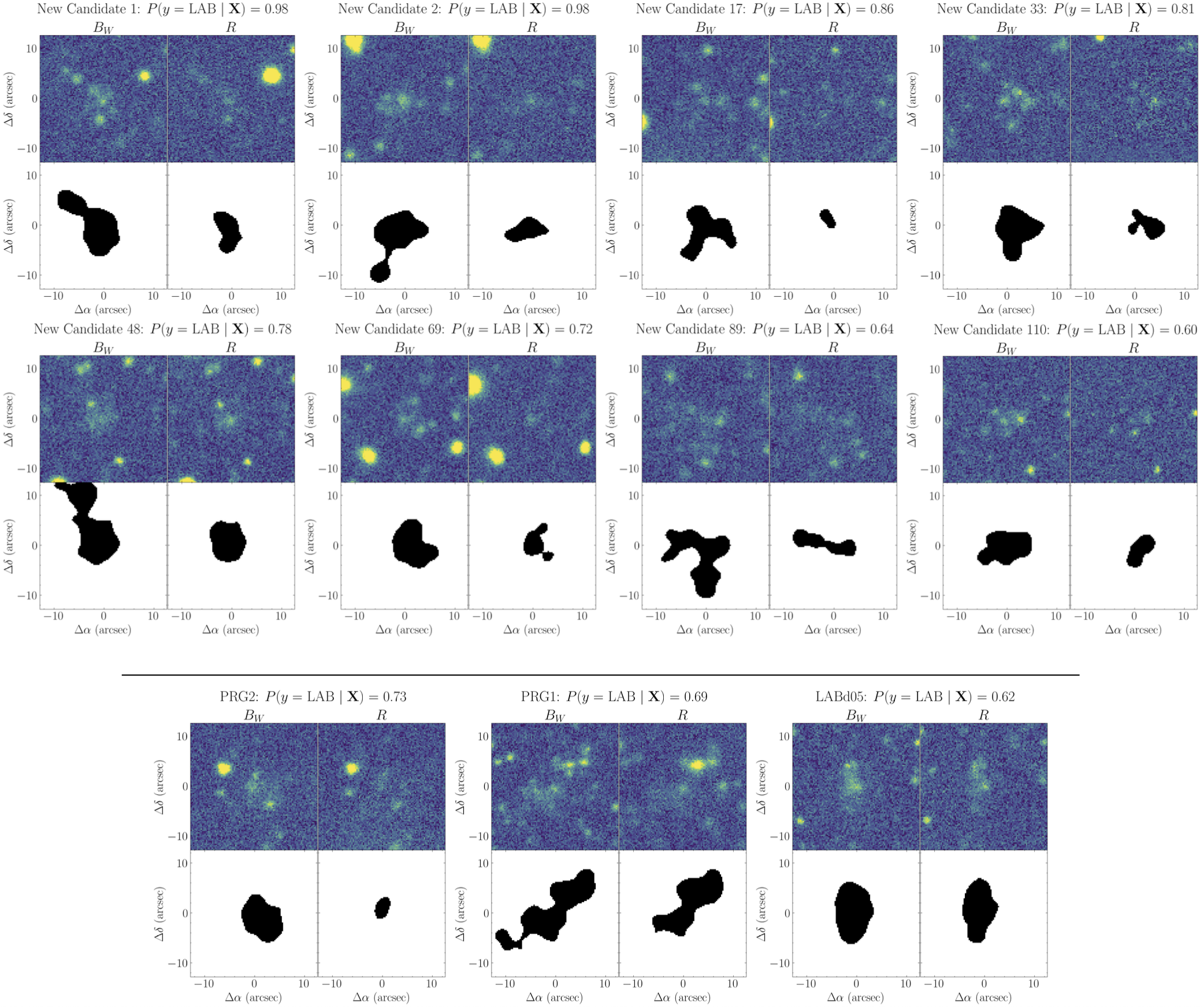
Narrowband LABs (Yang+09)
To evaluate how our pipeline performs when classifying LABs discovered via narrowband imaging, we identify the four LABs reported by Yang et al 2009 in the Boötes field. These objects are located in our master catalog, and their catalog data inlcuding images can be extracted using the following code.
import numpy as np
import pandas as pd
from astropy.io import fits
from astropy.stats import SigmaClip
from photutils.aperture import ApertureStats, CircularAnnulus
from pyBIA.data_processing import crop_image, concat_channels

# The path to the NDWFS data files
data_path_bw = 'NDWFS/fits_images/Bw_FITS/'
data_path_r = 'NDWFS/fits_images/R_FITS/'

# Load the candidate catalog according to the optimized model
cat = pd.read_csv('final_master_catalog.csv')

# The NDWFS Bootes catalog name and their names as they appear in the Yang+09 paper
yang_names = ['NDWFS_J142503.4+345854', 'NDWFS_J143059.0+353324', 'NDWFS_J143057.8+353431', 'NDWFS_J143725.0+351048']
yang_names_to_use = ['Yang+09 Blob 4', 'Yang+09 Blob 1', 'Yang+09 Blob 2', 'Yang+09 Blob 3']

# Find these in the master catalog
indices = []
for i in range(len(yang_names)):
        index = np.where(cat.obj_name == yang_names[i])[0]
        print(len(index))
        indices.append(index[0])

yang_sample = cat.iloc[indices]

# Saving images as 250x250 pix
image_size = 250

# Setting the apertures for the background subtraction, approximated using the sigma-clipped median within annuli of 20 and 35 pixel radii
annulus_apertures = CircularAnnulus((int(image_size/2),int(image_size/2)), r_in=20, r_out=35)

# Extract the images one field at a time, normalizing by the exposure time to convert to counts per second
counter = 0
images_bw, images_r = [], []
names = []
for field_name in np.unique(yang_sample['field_name']):

        # Load the B and R broadband data
        hdu_bw = fits.open(data_path_bw+field_name+'_Bw_03_fix.fits')
        hdu_r = fits.open(data_path_r+field_name+'_R_03_reg_fix.fits')

        # Select only the objects in this subfield
        subfield_index = np.where(yang_sample['field_name'] == field_name)[0]

        # Loop through these objects, subtract the background using aperture photometry, and save as txt file
        for i in range(len(subfield_index)):

                counter += 1
                print(counter)

                # Select the object's pixel positions
                xpix, ypix = yang_sample[['xpix', 'ypix']].iloc[subfield_index[i]].values.T

                # Bw first, crop the image from the entire subfield array, and calculate the background in this region
                image = crop_image(hdu_bw[0].data, x=np.array(xpix), y=np.array(ypix), size=image_size, invert=True)
                bkg_stats = ApertureStats(image, annulus_apertures, error=None, sigma_clip=SigmaClip())

                # Subtract the background and then normalize by the exposure time to get counts/sec
                image = (image - bkg_stats.median) / hdu_bw[0].header['EXPTIME']
                images_bw.append(image)

                # R next, crop the image from the entire subfield array, and calculate the background in this region
                image = crop_image(hdu_r[0].data, x=np.array(xpix), y=np.array(ypix), size=image_size, invert=True)
                bkg_stats = ApertureStats(image, annulus_apertures, error=None, sigma_clip=SigmaClip())

                # Subtract the background and then normalize by the exposure time to get counts/sec
                image = (image - bkg_stats.median) / hdu_r[0].header['EXPTIME']
                images_r.append(image)
                names.append(yang_sample.obj_name.iloc[subfield_index[i]])

#Confirmed that names == yang_names so these images are aligned with the csv
#NOW save
yang_images = concat_channels(np.array(images_bw), np.array(images_r))
np.save('Yang_Blob_Images.npy', yang_images)
yang_sample.to_csv('Yang_Blobs_Catalog.csv')
The dataframe containing the sub-catalog of these four narrowband-selected LABs, along with their corresponding images, can be downloaded below:
We now run these four objects through the iForest and CNN models to evaluate how all models classify each object, even if they were removed in the early XGBoost-based stage. Note that these scores are already included in the dataframe above; however, the code below demonstrates how the models were loaded and how these scores were calculated (except the initial XGBoost model, since all detected objects already have this score).
import numpy as np
import pandas as pd
from pyBIA import outlier_detection
from pyBIA.data_augmentation import resize

# FIRST DO THE OUTLIER DETECTION

image_size = 241 # Optimal image size to use
normalize = True
min_pixel = 0
max_pixel = 10
img_num_channels = 1
feat_set='hog'
clf = 'iforest'
impute = True
imp_method = 'median'
SEED_NO = 1909
#
model = outlier_detection.Classifier(
        normalize=normalize,
        min_pixel=min_pixel,
        max_pixel=max_pixel,
        img_num_channels=img_num_channels,
        feat_set=feat_set,
        clf=clf,
        impute=impute,
        imp_method=imp_method,
        SEED_NO=SEED_NO
        )

# Load the saved iForest model
model.load(path='anomaly_detection_model')

# CLASSIFY WITH iFOREST
yang_blobs = np.load('Yang_Blob_Images.npy')
yang_blobs = resize(yang_blobs, image_size)
iforest_predictions = model.predict(yang_blobs)

# Now add these iForest scores to the dataframe
yang_sample = pd.read_csv('Yang_Blobs_Catalog.csv')
yang_sample['iForest_scores'] = iforest_predictions[:,1]

# Now do the CNN
from pyBIA import cnn_model

# Load the saved model
model = cnn_model.Classifier()
model.load('cnn_model')

# Load the images and add the difference/color image
yang_blobs = np.load('Yang_Blob_Images.npy')
bw_minus_r = yang_blobs[:,:,:,0] / yang_blobs[:,:,:,1]
bw_minus_r = np.expand_dims(bw_minus_r, axis=-1)
yang_blobs = np.concatenate([yang_blobs, bw_minus_r], axis=-1)

# Now do the predictions
yang_cnn_predictions = model.predict(yang_blobs, cv_model='all', return_proba=True)

# Add the CNN score to the dataframe
yang_sample['CNN_proba'] = yang_cnn_predictions[:,1].astype('float')

# Now need to compute the Bw-R color to assess whether they would have made it through our priority selection
from astropy.io import fits
from pyBIA import catalog

data_path = 'NDWFS/fits_images/R_FITS/'

sig = 0.32 # The optimal noise-detection threshold to apply
frame = [] #To store all 27 subfields

# Loop through all the fields and save catalog
for fieldname in np.unique(np.array(yang_sample['field_name'])):

    # Load the field data
    data_hdu = fits.open(data_path+fieldname+'_R_03_reg_fix.fits')
    data_map, zeropoint, exptime = data_hdu[0].data, data_hdu[0].header['MAGZERO'], data_hdu[0].header['EXPTIME']

    subfield_index = np.where(yang_sample['field_name']==fieldname)[0]
    xpix, ypix = yang_sample[['xpix', 'ypix']].iloc[subfield_index].values.T
    objname, field, flag = yang_sample[['obj_name', 'field_name', 'flag']].iloc[subfield_index].values.T

    # Create the catalog object
    cat = catalog.Catalog(data_map, error=None, x=xpix, y=ypix, zp=zeropoint, exptime=exptime, nsig=sig, flag=flag, obj_name=objname, field_name=field, invert=True)

    # Generate the catalog and save the subfield catalog, after which it is appended to the master frame
    cat.create(save_file=False)#, filename='Cat_BW_Subfield_'+fieldname)
    frame.append(cat.cat)

# Combine all 27 sub-catalogs into one master frame and save
frame = pd.concat(frame, axis=0, join='inner')

# NOW FRAME IS SAME ORDER AS YANG_SAMPLE CSV
# Add Bw-R color to the dataframe
yang_sample['Color'] = np.array(yang_sample.mag) - np.array(frame.mag)

# FINAL SAVE FOR YANG CSV
yang_sample.to_csv('Yang_Blobs_Catalog.csv')
With all machine learning probability predictions calculated, we now plot the narrowband-selected LABs, displaying their scores above each image.
from pyBIA import catalog
import pandas as pd
import numpy as np
from pyBIA.data_augmentation import resize
import matplotlib.pyplot as plt
import scienceplots
plt.style.use('science')
plt.rcParams.update({'font.size':21,})

# Load the images and resize to 100x100 pixels
yang_blob_images = np.load('Yang_Blob_Images.npy')
yang_blob_images = resize(yang_blob_images, 100)

# To store the segmentation patches
yang_blob_images_bw, yang_blob_images_r = [], []
yang_blob_images_segm1, yang_blob_images_segm2 = [], []
for i in range(4):
    data1 = np.flip(yang_blob_images[:,:,:,0][i], axis=0)
    data2 = np.flip(yang_blob_images[:,:,:,1][i], axis=0)
    segm1_ = catalog.get_segmentation(data1, nsig=0.32, xpix=None, ypix=None, size=100, median_bkg=0)
    segm2_ = catalog.get_segmentation(data2, nsig=0.32, xpix=None, ypix=None, size=100, median_bkg=0)
    yang_blob_images_segm1.append(segm1_), yang_blob_images_segm2.append(segm2_)
    yang_blob_images_bw.append(data1); yang_blob_images_r.append(data2)

yang_blob_images_bw, yang_blob_images_r = np.array(yang_blob_images_bw), np.array(yang_blob_images_r)

# Load the catalog and store the XGBoost-8 and CNN probability predictions
df_yang = pd.read_csv('Yang_Blobs_Catalog.csv')
names = ['Yang+09 Blob 4', 'Yang+09 Blob 1', 'Yang+09 Blob 2', 'Yang+09 Blob 3']
probas_xgb = np.array(df_yang.XGBoost8_Proba)
probas_cnn = np.array(df_yang.CNN_proba)

# PLOT
pix_conversion = 3.8961 # NDWFS pixel-per-arcsecond conversion factor
image_size = 100 # Image size (100x100 pixels)

# Create pixel grids centered at (50, 50)
x = np.arange(0, image_size) - image_size // 2 # Shift by 50 to center at (0,0)
y = np.arange(0, image_size) - image_size // 2

# Convert pixel coordinates to arcseconds
x_arcsec = x / pix_conversion
y_arcsec = y / pix_conversion

for i in range(4):

    # Calculate vmin/vmax (robust scale)
    data = yang_blob_images_bw[i]
    index = np.where(np.isfinite(data))
    std = np.median(np.abs(data[index] - np.median(data[index])))
    vmin = np.median(data[index]) - 3 * std
    vmax = np.median(data[index]) + 10 * std

    # Calculate vmin/vmax (robust scale)
    data = yang_blob_images_r[i]
    index = np.where(np.isfinite(data))
    std = np.median(np.abs(data[index] - np.median(data[index])))
    vminr = np.median(data[index]) - 3 * std
    vmaxr = np.median(data[index]) + 10 * std

    fig, ax = plt.subplots(nrows=2, ncols=2, figsize=(8, 8), sharex=True, sharey=True)

    # Plot images with arcsecond scaling for the axes
    im1 = ax[0, 0].imshow(yang_blob_images_bw[i], vmin=vmin, vmax=vmax, cmap='viridis', extent=[x_arcsec.min(), x_arcsec.max(), y_arcsec.min(), y_arcsec.max()])
    im2 = ax[0, 1].imshow(yang_blob_images_r[i], vmin=vminr, vmax=vmaxr, cmap='viridis', extent=[x_arcsec.min(), x_arcsec.max(), y_arcsec.min(), y_arcsec.max()])
    im3 = ax[1, 0].imshow(yang_blob_images_segm1[i], cmap='binary', extent=[x_arcsec.min(), x_arcsec.max(), y_arcsec.min(), y_arcsec.max()])
    im4 = ax[1, 1].imshow(yang_blob_images_segm2[i], cmap='binary', extent=[x_arcsec.min(), x_arcsec.max(), y_arcsec.min(), y_arcsec.max()])

    ax[0, 0].set_title(r'$B_W$')
    ax[0, 1].set_title(r'$R$')

    fig.suptitle(f'{names[i]}\n$P(y =$ LAB $\mid \\mathbf{{X}})$ = {probas_xgb[i]:.2f} (XGBoost) \& {probas_cnn[i]:.2f} (CNN)', y=1.02)

    plt.subplots_adjust(wspace=0, hspace=0)

    ax[0, 0].set_ylabel(r'$\Delta \delta$ (arcsec)')
    ax[1, 0].set_ylabel(r'$\Delta \delta$ (arcsec)')
    ax[1, 0].set_xlabel(r'$\Delta \alpha$ (arcsec)')
    ax[1, 1].set_xlabel(r'$\Delta \alpha$ (arcsec)')

    plt.savefig(f'YANG_{i}.png', dpi=300, bbox_inches='tight')
    plt.show()
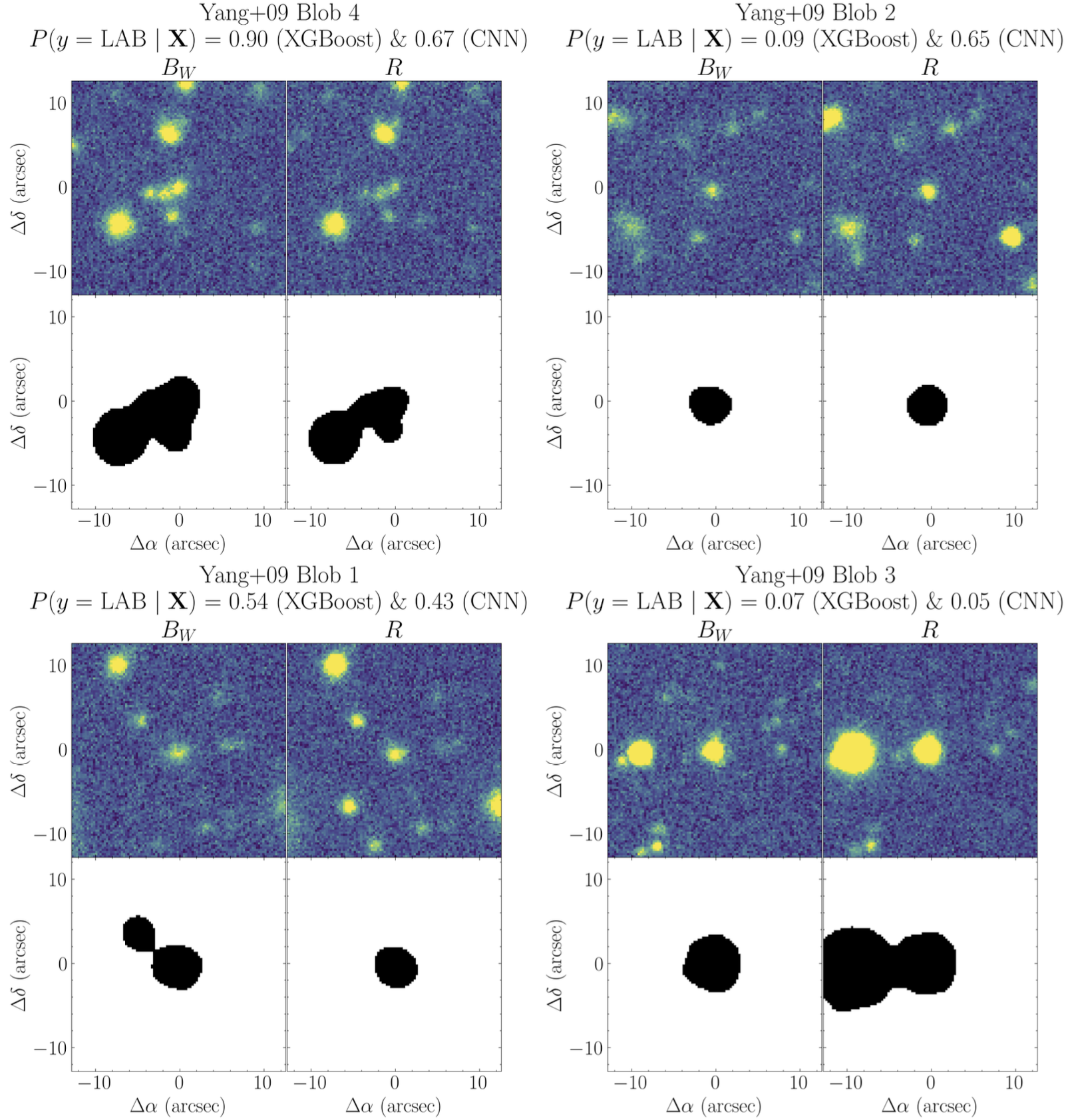
Finally, we compare these four narrowband-selected LABs with the broadband-selected LABs from our training set.
import pandas as pd
import numpy as np
import matplotlib.pyplot as plt
from matplotlib.lines import Line2D
import scienceplots  # for plot style
plt.style.use("science")
plt.rcParams.update({"font.size": 21})

pix_conversion = 3.8961  # NDWFS pixel-per-arcsecond conversion factor

# Load the catalogs
master_cat = pd.read_csv('final_master_catalog.csv')
confirmed_names = np.loadtxt('confirmed_diffuse_names.txt', dtype=str)

indices = []
for i in range(len(confirmed_names)):
    index = np.where(master_cat.obj_name == confirmed_names[i])[0]
    indices.append(index[0])
    print(len(index))

# Index the master catalog to only the confirmed LABs
master_cat = master_cat.iloc[indices]

# Set the attributes to plot
lab_bw_mag = np.array(master_cat.mag)
lab_area = np.array(master_cat.area)
lab_gini = np.array(master_cat.gini)
lab_BW_minus_R = np.array(master_cat.Color)
lab_cnn = np.array(master_cat.CNN_proba)
lab_xgb = np.array(master_cat.XGBoost8_Proba)
lab_names = ['PRG4', 'LABd05', 'PRG3', 'PRG2', 'PRG1']

# Load the Yang+09 catalog and set the attributes
df_yang = pd.read_csv("Yang_Blobs_Catalog.csv")
yang_bw_mag = np.array(df_yang.mag)
yang_bw_area = np.array(df_yang.area)
yang_bw_gini = np.array(df_yang.gini)
yang_BW_minus_R = np.array(df_yang.Color)
yang_cnn = np.array(df_yang.CNN_proba)
yang_xgb = np.array(df_yang.XGBoost8_Proba)
yang_names_to_use = ['Yang+09 Blob 4', 'Yang+09 Blob 1', 'Yang+09 Blob 2', 'Yang+09 Blob 3']

# Set up colormap and normalization (for probability values ranging from 0 to 1)
cmap = plt.get_cmap('viridis')
norm = plt.Normalize(0, 1)

# PLOT
special_colors_lab = ['red', 'blue', 'purple', 'cyan', 'green']
special_markers_lab = ['^', 'p',  'v', '>', 'P']

special_colors_yang = ['orange', 'magenta', 'brown', 'olive']
special_markers_yang = ['s', 'd', 'h', 'X']  # square, thin diamond, hexagon, star

# Set up colormap and normalization (probabilities range from 0 to 1)
cmap = plt.get_cmap('viridis')
norm = plt.Normalize(0, 1)

# To control marker size and linewidths (the Yang+09 LABs have thinner markerlines)
SS = 850
LW_BLOB = 7
LW_YANG = 2

fig, (ax1, ax2) = plt.subplots(ncols=2, figsize=(16,8))

# Left subplot
# Plot confirmed LAB in our training set
for i in range(len(lab_names)):
    print('LAB:',i)
    print(lab_names[i], special_markers_lab[i], special_colors_lab[i])
    ax1.scatter(lab_gini[i],
                lab_area[i]/pix_conversion**2,
                marker=special_markers_lab[i],
                s=SS,
                linewidth=LW_BLOB,
                alpha=0.9,
                c=[lab_xgb[i]], # face color determined by XGB probability
                cmap=cmap,
                norm=norm,
                edgecolor=special_colors_lab[i])

# Plot Yang+09 LABs
for i in range(len(yang_names_to_use)):
    ax1.scatter(yang_bw_gini[i],
                yang_bw_area[i]/pix_conversion**2,
                marker=special_markers_yang[i],
                s=SS,
                linewidth=LW_YANG,
                alpha=0.9,
                c=[yang_xgb[i]], # face color determined by XGB probability
                cmap=cmap,
                norm=norm,
                edgecolor=special_colors_yang[i])

ax1.set_ylabel(r'$B_W$ Area (arcsec$^2$)')
ax1.set_xlabel('Gini Index')

# Right Subplot
# Plot confirmed LAB in our training set
for i in range(len(lab_names)):
    ax2.scatter(lab_cnn[i],
                lab_BW_minus_R[i],
                marker=special_markers_lab[i],
                s=SS,
                linewidth=LW_BLOB,
                alpha=0.9,
                c=[lab_xgb[i]], # face color determined by XGB probability
                cmap=cmap,
                norm=norm,
                edgecolor=special_colors_lab[i])

# Plot Yang+09 LABs
for i in [1, 3, 2, 0]:
    ax2.scatter(yang_cnn[i],
                yang_BW_minus_R[i],
                marker=special_markers_yang[i],
                s=SS,
                linewidth=LW_YANG,
                alpha=0.9,
                c=[yang_xgb[i]], # face color determined by XGB probability
                cmap=cmap,
                norm=norm,
                edgecolor=special_colors_yang[i])

ax2.set_xlabel('CNN Probability Prediction')
ax2.set_ylabel(r'$B_W - R$')

#Shared custom legend
row1 = ['LABd05', 'PRG1', 'PRG2', 'PRG3', 'PRG4']
row2 = ['Yang+09 Blob 1', 'Yang+09 Blob 2', 'Yang+09 Blob 3', 'Yang+09 Blob 4']

# Map names -> style indices
lab_idx  = {name: i for i, name in enumerate(lab_names)}
yang_idx = {name: i for i, name in enumerate(yang_names_to_use)}

def handle_for(name):
    # Quick function to return legend handle according to the object name (to distinguish between the LAB types)
    if name in lab_idx:
        i = lab_idx[name]
        return Line2D([0], [0], marker=special_markers_lab[i], color='w',
                      markerfacecolor="none", markeredgecolor=special_colors_lab[i],
                      markersize=20, markeredgewidth=5)
    else:
        i = yang_idx[name]
        return Line2D([0], [0], marker=special_markers_yang[i], color='w',
                      markerfacecolor="none", markeredgecolor=special_colors_yang[i],
                      markersize=20, markeredgewidth=2)

handles, labels = [], []
ncols = 5
for j in range(ncols):
    if j < len(row1):
        handles.append(handle_for(row1[j])); labels.append(row1[j])
    if j < len(row2):
        handles.append(handle_for(row2[j])); labels.append(row2[j])

fig.legend(handles=handles, labels=labels,
           loc='upper center', ncol=ncols, frameon=True, fancybox=True,
           bbox_to_anchor=(0.5, 1.05))

# Shared colorbar
sm = plt.cm.ScalarMappable(cmap=cmap, norm=norm)
sm.set_array([])

cbar_ax = fig.add_axes([0.90, 0.15, 0.02, 0.7])

cbar = fig.colorbar(sm, cax=cbar_ax)
cbar.set_label('XGBoost Probability Prediction')

plt.tight_layout(rect=[0, 0, 0.9, 0.95])
plt.savefig('lab_yang_comparison_scatter.png', dpi=300, bbox_inches='tight')
plt.show()
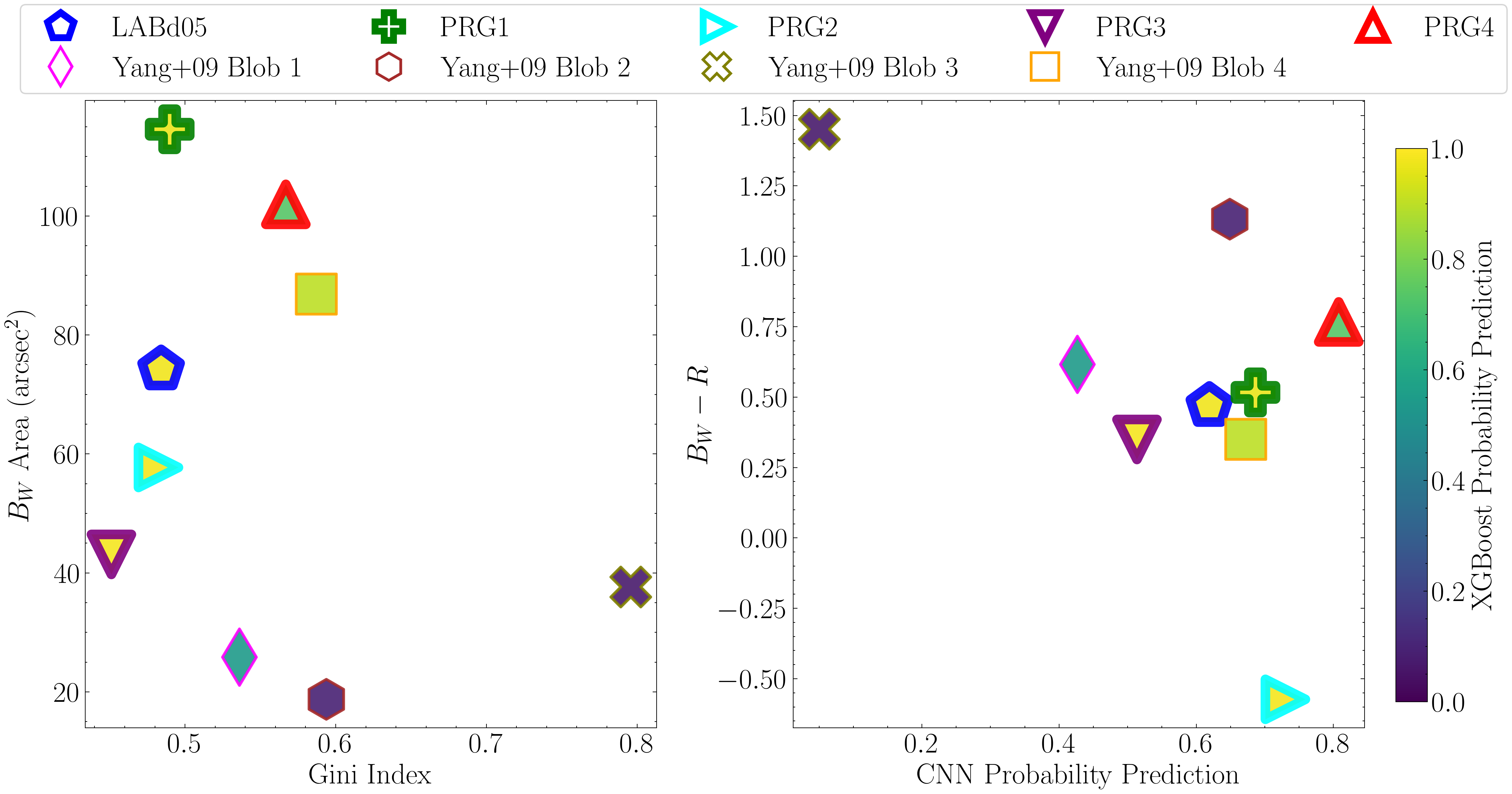
Candidate Table and Image Cutouts
Below, we provide the code used to generate the final table presented in the paper (Table 5) along with the corresponding imaging cutouts shown in Fig. 14.
import numpy as np
import pandas as pd
from astropy.coordinates import SkyCoord
from astropy import units as u

final_cat = pd.read_csv('Final_New_Candidate_Catalog.csv')

# sort by CNN probability
sort_index = np.argsort(final_cat.CNN_proba)[::-1]
final_cat = final_cat.iloc[sort_index]

final_names = np.array([name.replace('_', '') for name in final_cat.obj_name])
final_cnn_probas = np.array(final_cat.CNN_proba)
final_xgb_probas = np.array(final_cat.XGBoost8_Proba)

for i in range(len(final_cat)):

    # Convert the coordinates which are stored in the catalog in decimal degrees
    ra_decimal, dec_decimal = final_cat.ra.iloc[i], final_cat.dec.iloc[i]
    c = SkyCoord(ra=ra_decimal*u.degree, dec=dec_decimal*u.degree)
    ra_str, dec_str = c.to_string('hmsdms', precision=3).split()

    # For readibility
    ra_hms = ra_str.replace('h', ':').replace('m', ':').replace('s', '')
    dec_dms = dec_str.replace('+', '').replace('d', ':').replace('m', ':').replace('s', '')

    # This is formatted for easy placement in the LaTex table (Table 5 of the paper)
    print(fr'({i+1}) & {final_names[i]} & {ra_hms} & {dec_dms} & '
      f'{final_cnn_probas[i]:.2f} & '
      f'{final_cat.mag.iloc[i]:.2f} $\pm$ {final_cat.mag_err.iloc[i]:.2f} & '
      f'{final_cat.Color.iloc[i]:.2f} \\\\')
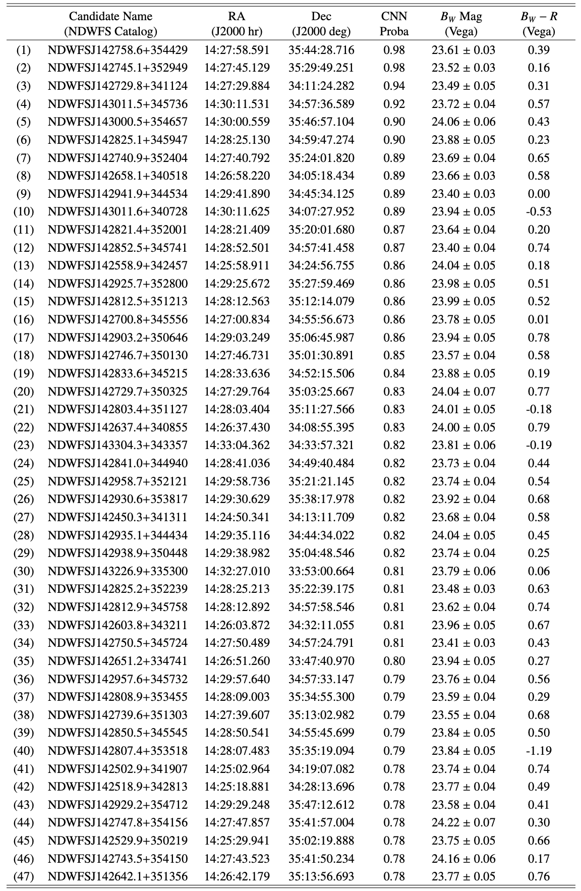
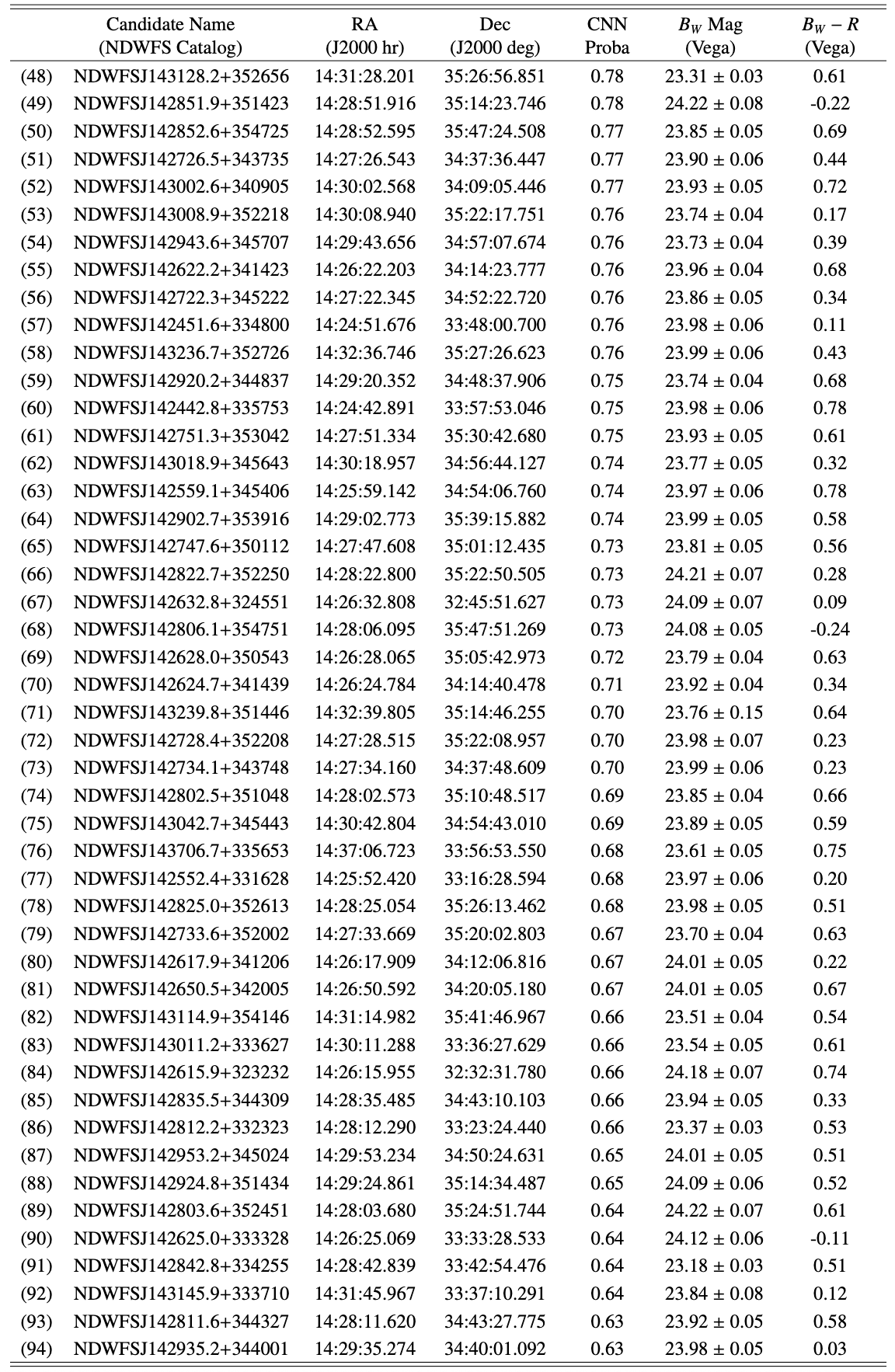
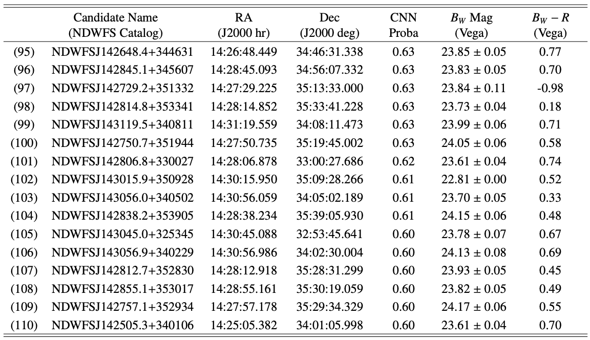
import numpy as np
import matplotlib.pyplot as plt
import matplotlib.gridspec as gridspec
import pandas as pd
import scienceplots
from pyBIA.data_augmentation import resize
plt.style.use('science')
plt.rcParams.update({'font.size': 21})

# Load the priority candidate catalog
final_cat = pd.read_csv('Final_New_Candidate_Catalog.csv')
final_cnn_probas = np.array(final_cat.CNN_proba)
final_images = np.load('Final_New_Candidate_Images.npy')
final_images = resize(final_images, 100) # Resize to 100x100 pixels

# Sort the objects based on the CNN probability prediction score
x = np.argsort(final_cnn_probas)[::-1]
final_images = final_images[x]
final_cnn_probas = final_cnn_probas[x]

n_select = len(final_cnn_probas) # Number of priority candidates (110)

# For plotting/setting axes
pix_conversion = 3.8961  # NDWFS pixel/arcsec
image_size = 100
x = np.arange(image_size) - image_size // 2
y = np.arange(image_size) - image_size // 2
x_arcsec = x / pix_conversion
y_arcsec = y / pix_conversion

# Loop through and plot all individually
for i in range(n_select):

    # All this time we have been flipping images to be North-up
    bw_img = np.flip(final_images[i, :, :, 0], axis=0)
    r_img = np.flip(final_images[i, :, :, 1], axis=0)

    # Bw image with robust scaling for vmin/vmax
    data = bw_img
    valid = np.isfinite(data)
    std = np.median(np.abs(data[valid] - np.median(data[valid])))
    vmin = np.median(data[valid]) - 3 * std
    vmax = np.median(data[valid]) + 10 * std

    # R image with robust scaling for vmin/vmax
    datar = r_img
    validr = np.isfinite(datar)
    stdr = np.median(np.abs(datar[validr] - np.median(datar[validr])))
    vminr = np.median(datar[valid]) - 3 * stdr
    vmaxr = np.median(datar[valid]) + 10 * stdr

    # PLOT
    fig = plt.figure(figsize=(16, 8))
    gs = gridspec.GridSpec(2, 1, height_ratios=[1, 1], hspace=0.02)

    ax1 = fig.add_subplot(gs[0])
    ax2 = fig.add_subplot(gs[1], sharex=ax1, sharey=ax1)

    im1 = ax1.imshow(bw_img, cmap='viridis', vmin=vmin, vmax=vmax,
                     extent=[x_arcsec.min(), x_arcsec.max(), y_arcsec.min(), y_arcsec.max()])
    im2 = ax2.imshow(r_img, cmap='viridis', vmin=vminr, vmax=vmaxr,
                     extent=[x_arcsec.min(), x_arcsec.max(), y_arcsec.min(), y_arcsec.max()])

    ax1.text(0.02, 0.95, r'$B_W$', color='white', transform=ax1.transAxes,
             fontsize=20, verticalalignment='top', horizontalalignment='left')
    ax2.text(0.02, 0.95, r'$R$', color='white', transform=ax2.transAxes,
             fontsize=20, verticalalignment='top', horizontalalignment='left')

    ax1.set_xticklabels([])
    ax1.set_yticklabels([])
    ax2.set_xticklabels([])
    ax2.set_yticklabels([])

    ax1.set_title(f'({i+1})')

    plt.setp(ax1.get_xticklabels(), visible=False)
    plt.subplots_adjust(hspace=0.03)
    plt.savefig(f'({i+1}).png', dpi=300, bbox_inches='tight')
    plt.close()
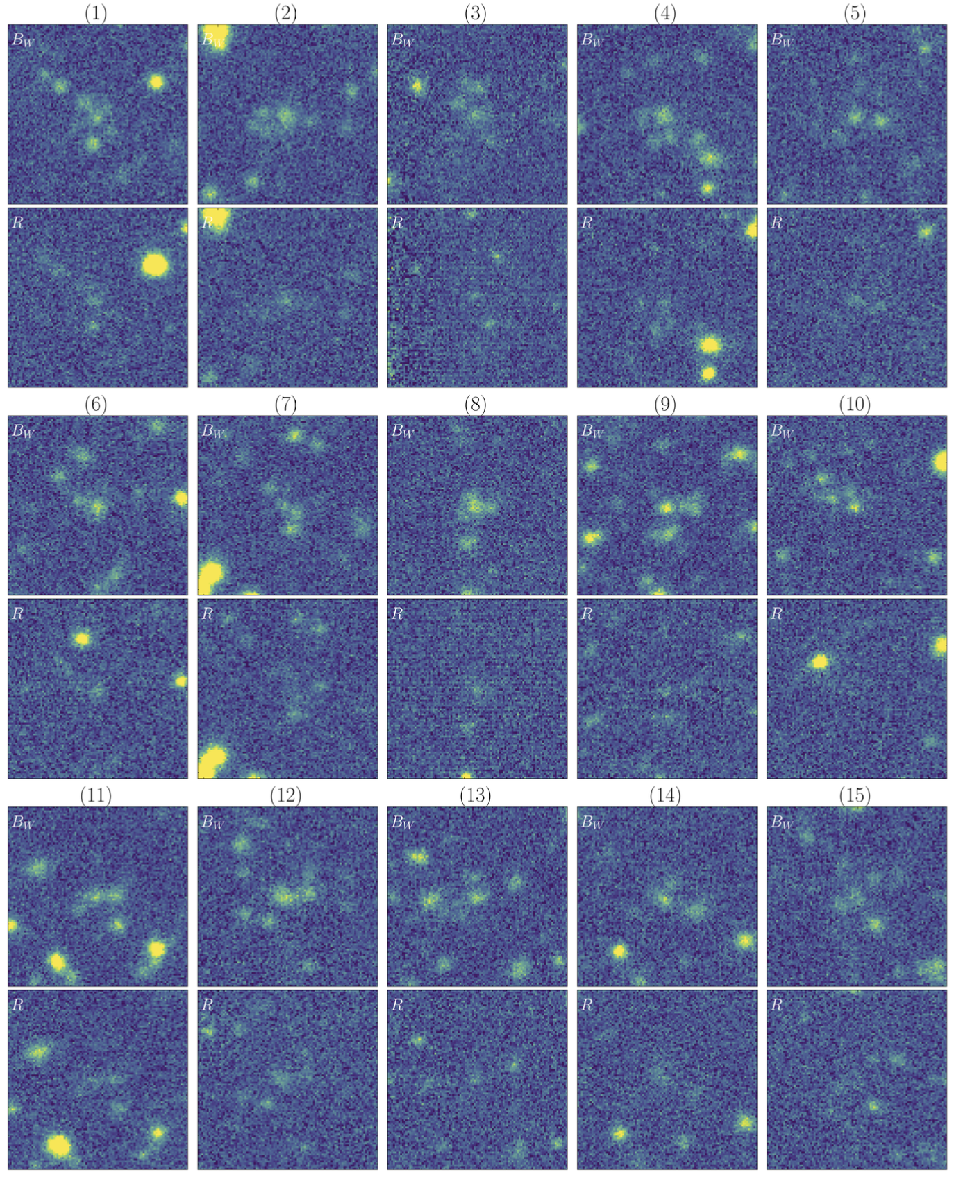
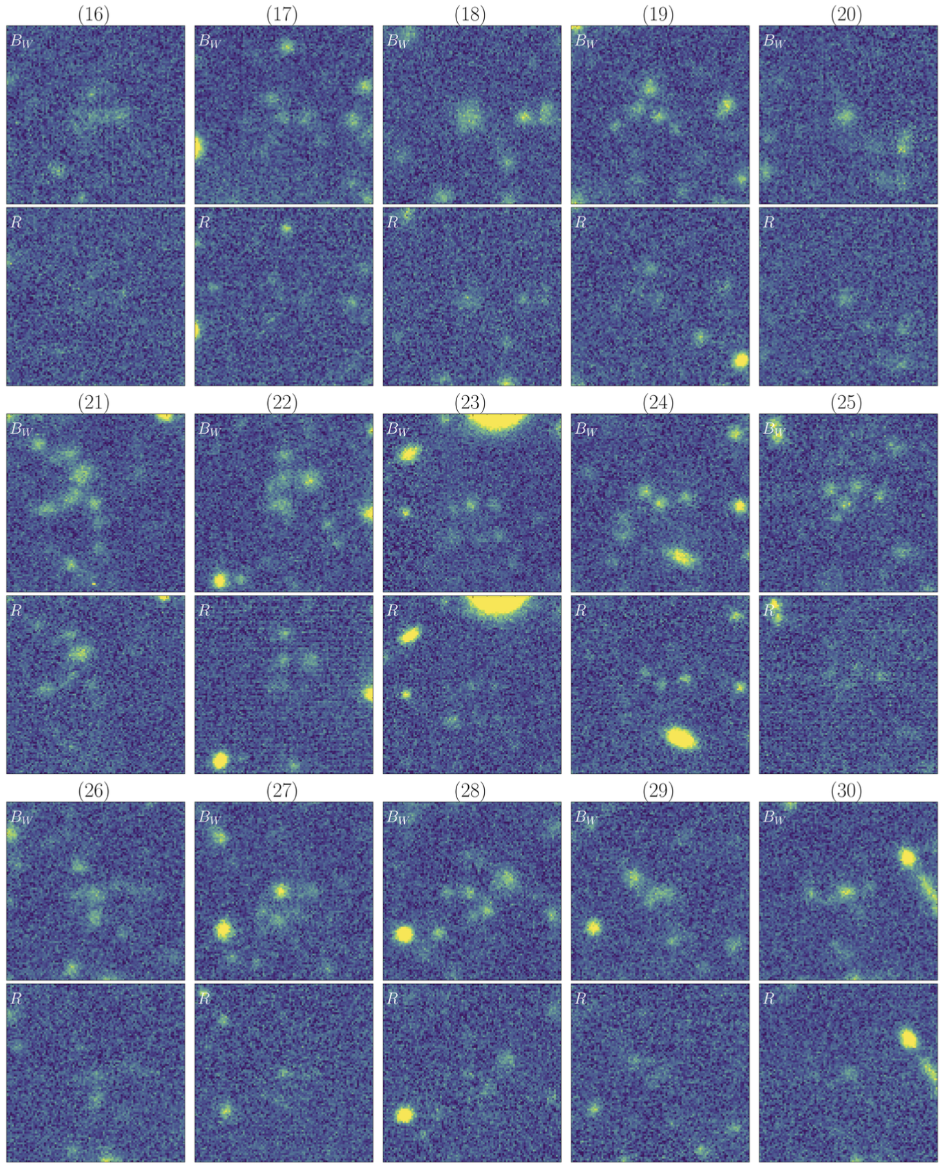
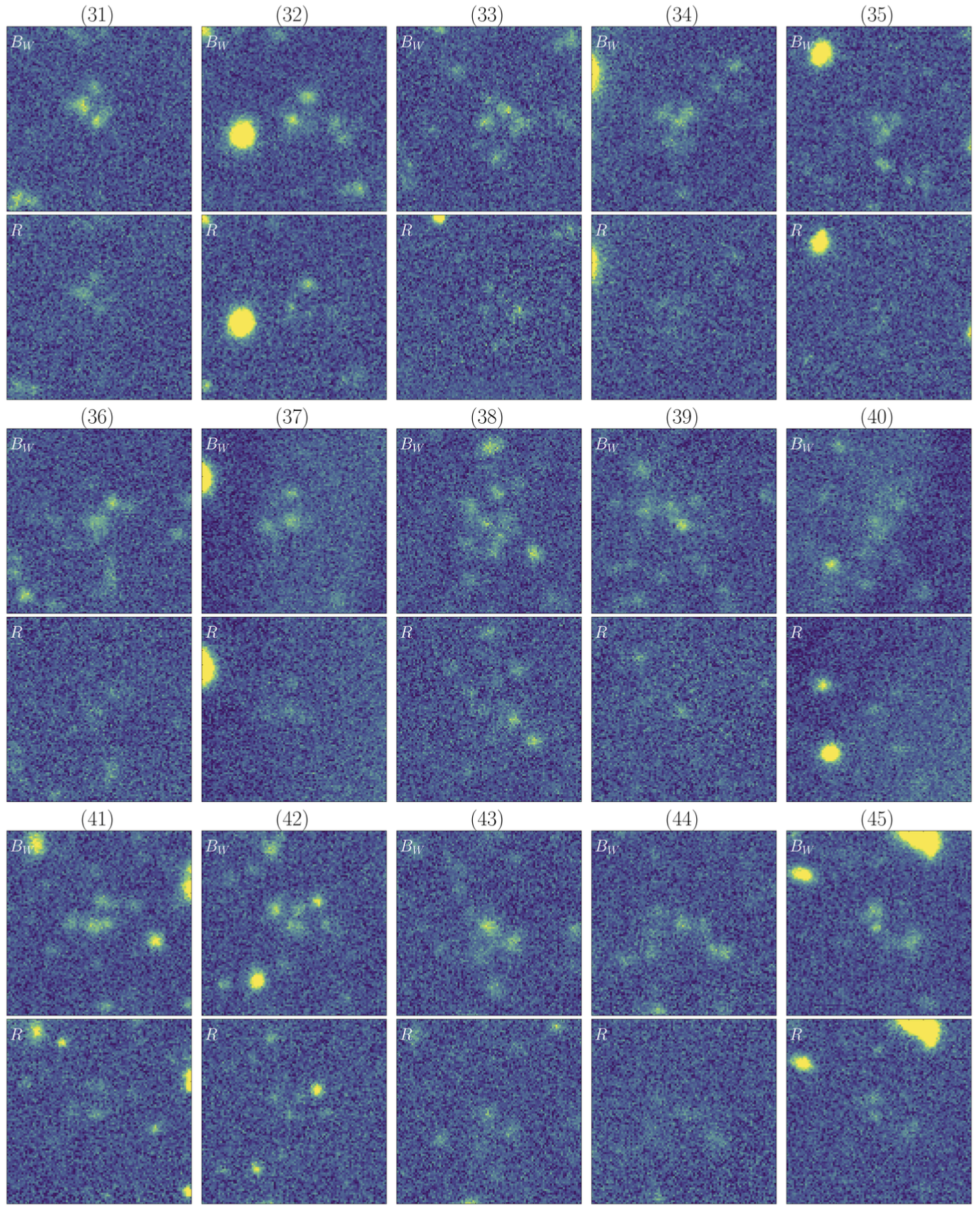
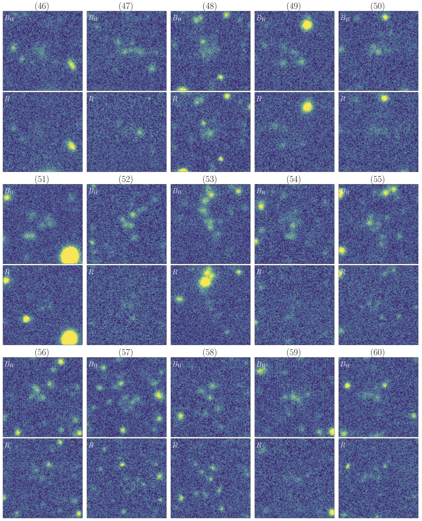
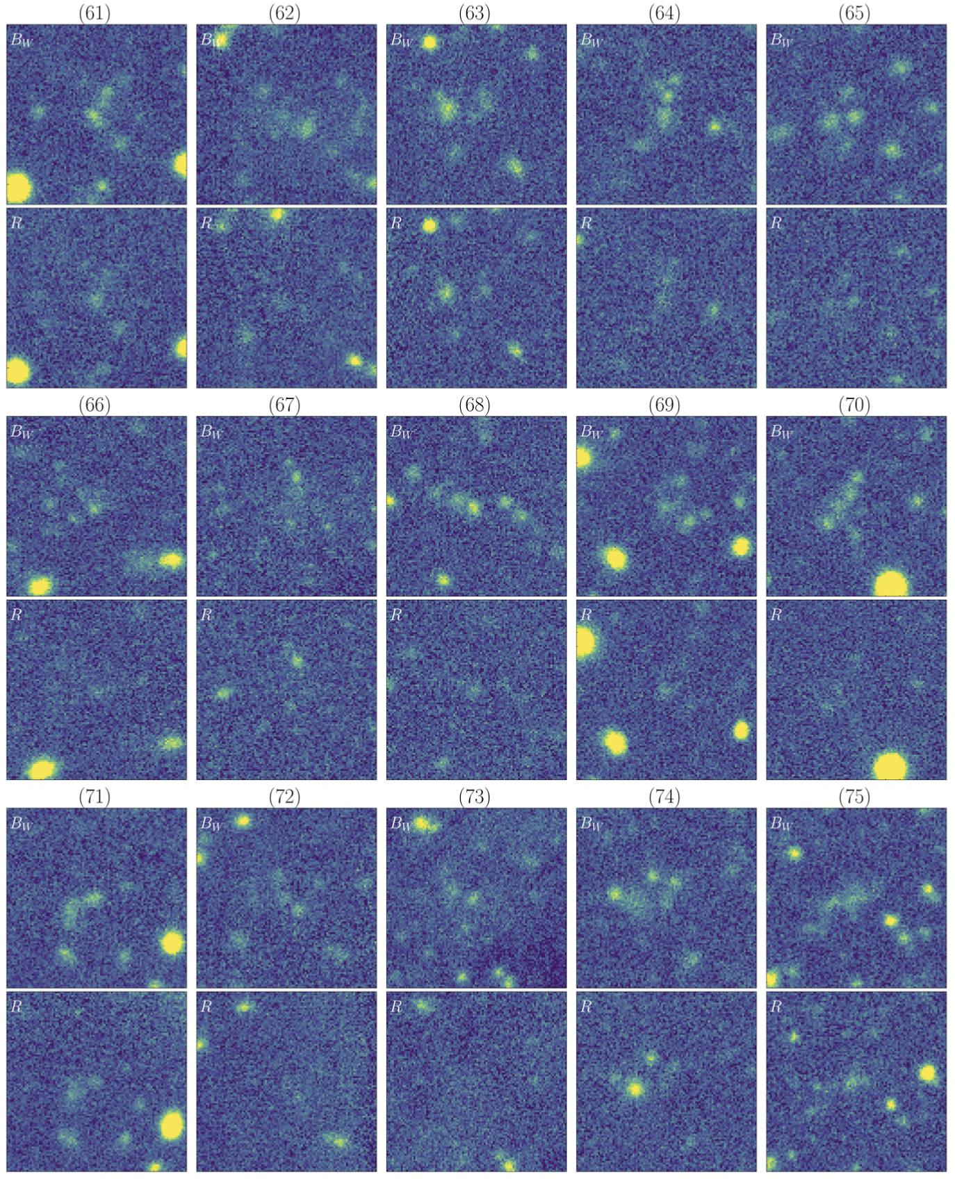
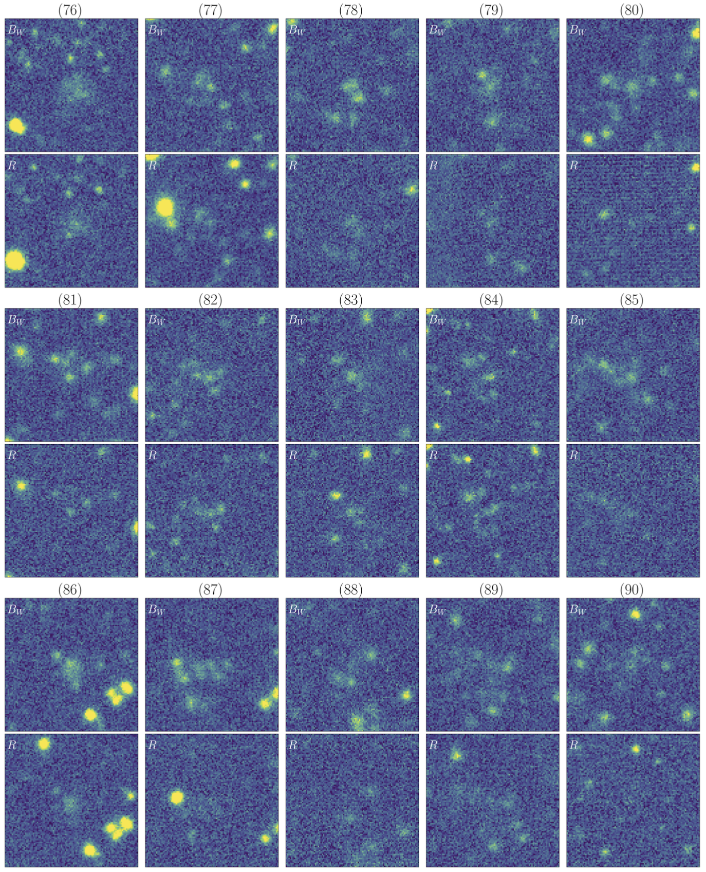
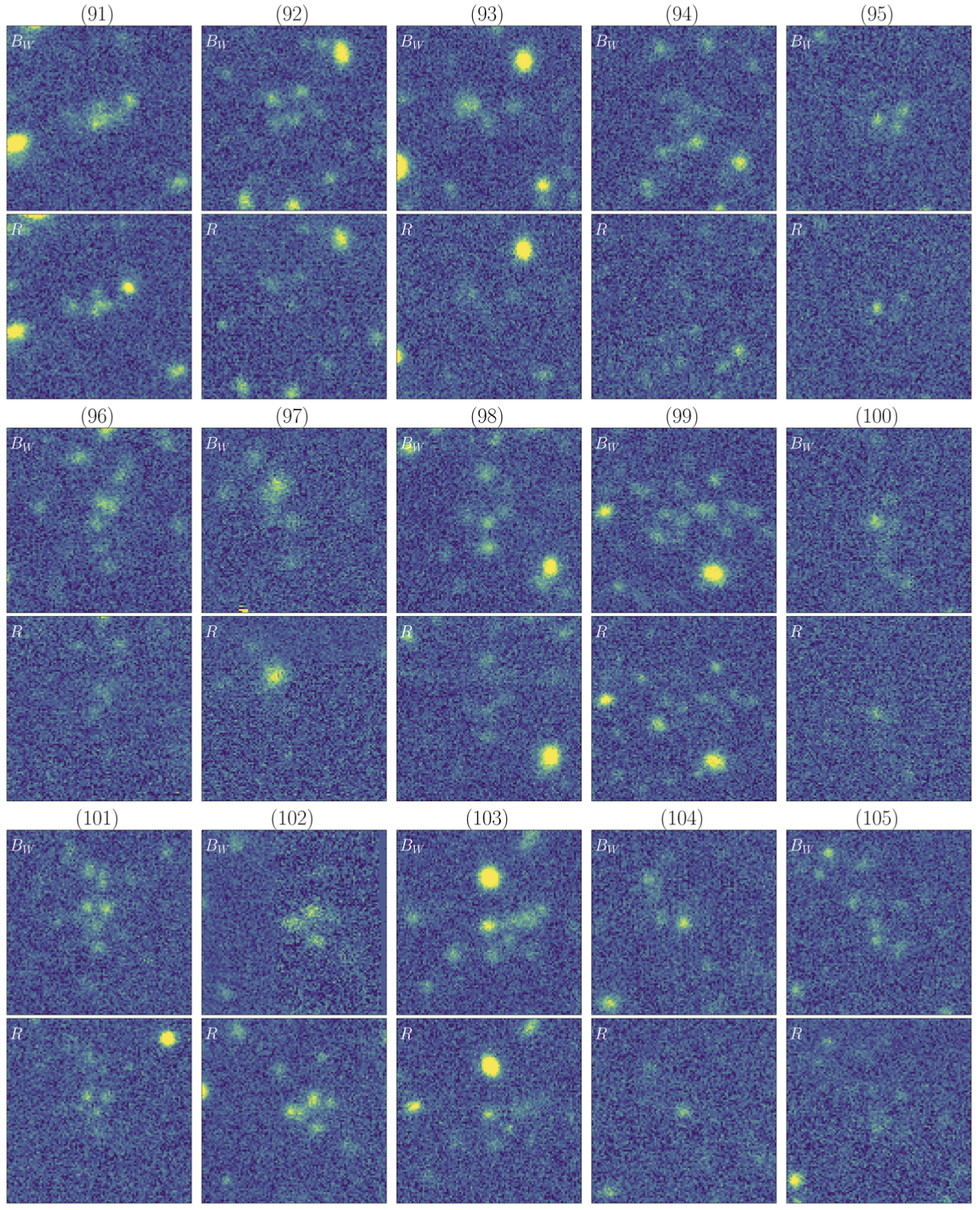
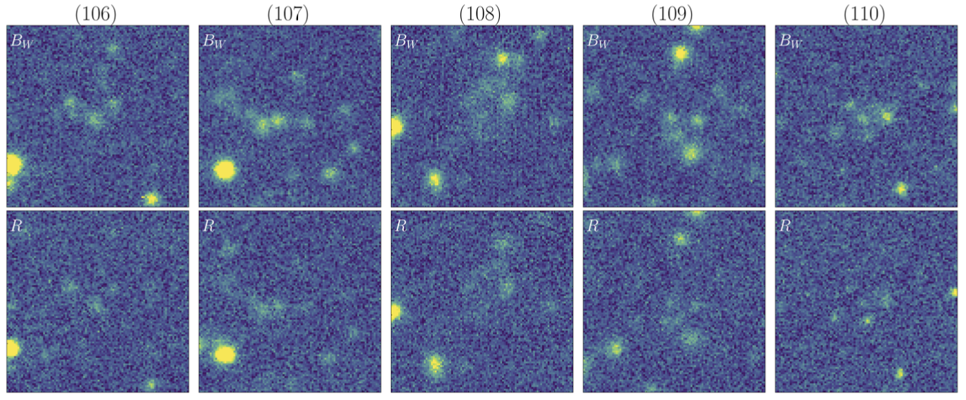
Appendix: Morphology Only Model
Here we present the results of an XGBoost model trained only on the segmentation-based morphological descriptors. As such, the feature matrix used to train this model does not include the Bw Mag and corresponding error, as well as the min and max pixel value within the segmentation. Using the same segmentation detection threshold of 0.32, this model is tuned using the same optimization routine used to train XGBoost-8.
import numpy as np
import pandas as pd
from pyBIA import ensemble_model, data_processing

sig = 0.32 # The optimal sig threshold to apply as per Figure 2
df = pd.read_csv('nsigs/_Bw_training_set_nsig_'+str(sig))
hu_cols = ['Hu1', 'Hu2', 'Hu3', 'Hu4', 'Hu5', 'Hu6', 'Hu7']
df[hu_cols] = df[hu_cols].apply(data_processing.signed_log_transform)

# Omit any non-detections
mask = np.where((df['area'] != -999) & np.isfinite(df['mag']) & np.all(np.isfinite(df[[f'Hu{i}' for i in range(1, 8)]]), axis=1))[0]

# Balance both classes to be of same size
blob_index = np.where(df['flag'].iloc[mask] == 1)[0]
other_index = np.where(df['flag'].iloc[mask] == 0)[0]
df_filtered = df.iloc[mask[np.concatenate((blob_index, other_index[:len(blob_index)]))]]

#These are the features to use, note that the catalog includes more than this!
# NOTE: Removing mag, mag_err, max_value, and min_value
columns = [
    #'mag', 'mag_err',
    'M00', 'M10', 'M01', 'M20', 'M11', 'M02', 'M30', 'M21', 'M12', 'M03',
    'mu20', 'mu11', 'mu02', 'mu30', 'mu21', 'mu12', 'mu03',
    'G10', 'G01', 'G20', 'G11', 'G02', 'G30', 'G21', 'G12', 'G03',
    'Hu1', 'Hu2', 'Hu3', 'Hu4', 'Hu5', 'Hu6', 'Hu7',
    'L00', 'L10', 'L01', 'L20', 'L11', 'L02', 'L30', 'L21', 'L12', 'L03',
    'area', 'covar_sigx2', 'covar_sigy2', 'covar_sigxy', 'covariance_eigval1', 'covariance_eigval2',
    'cxx', 'cxy', 'cyy', 'eccentricity', 'ellipticity', 'elongation',
    'equivalent_radius', 'fwhm', 'gini', 'orientation', 'perimeter',
    'semimajor_sigma', 'semiminor_sigma'#, 'max_value', 'min_value'
]

# Training data arrays
data_x, data_y = np.array(df_filtered[columns]), np.array(df_filtered['flag'])

# XGB-BASED BorutaSHAP
SEED_NO = 1909 # The seed number that will initialize the stochastic process (e.g., model training)
clf = 'xgb' # The classification model that will be trined, options are: 'xgb', 'rf' and 'nn'
impute = False # Whether to impute missing values (NaN)
optimize = True # Will enable the optimization routine
scoring_metric = 'f1' # The optimization trials will be assessed according to the F1 Score
opt_cv = 10 # The number of folds to perform during cross validation, ONLY used during optimization (`optimize`=True)
boruta_trials = 100 # Number of feature selection trials to perform (This is fast especially with `boruta_model`='xgb')
boruta_model = 'xgb' # The model to use when assessing feautre importances during feature selection (either 'rf' or 'xgb', DOES NOT have to match the `clf`)
n_iter = 100 # Number of hyperparameter optimization trials to perform, can set to 0 to disable hyperparam tuning
limit_search = True # Set to False to expand the hyperparameter search space (will take longer)

model = ensemble_model.Classifier(
    data_x,
    data_y,
    clf=clf,
    impute=impute,
    optimize=optimize,
    boruta_trials=boruta_trials,
    boruta_model=boruta_model,
    n_iter=n_iter,
    scoring_metric=scoring_metric,
    opt_cv=opt_cv,
    limit_search=limit_search,
    SEED_NO=SEED_NO
    )

model.create()
model.save('XGBoost_Morph_Only')

# The feature importance plot! Commenting out non-morph features
columns_formatted = [
    #r'$B_W$ Mag', r'$B_W$ MagErr',
    r'$M_{00}$', r'$M_{10}$', r'$M_{01}$', r'$M_{20}$', r'$M_{11}$', r'$M_{02}$', r'$M_{30}$', r'$M_{21}$', r'$M_{12}$', r'$M_{03}$',
    r'$\mu_{20}$', r'$\mu_{11}$', r'$\mu_{02}$', r'$\mu_{30}$', r'$\mu_{21}$', r'$\mu_{12}$', r'$\mu_{03}$',
    r'$G_{10}$', r'$G_{01}$', r'$G_{20}$', r'$G_{11}$', r'$G_{02}$', r'$G_{30}$', r'$G_{21}$', r'$G_{12}$', r'$G_{03}$',
    r'$h_1$', r'$h_2$', r'$h_3$', r'$h_4$', r'$h_5$', r'$h_6$', r'$h_7$',
    r'$L_{00}$', r'$L_{10}$', r'$L_{01}$', r'$L_{20}$', r'$L_{11}$', r'$L_{02}$', r'$L_{30}$', r'$L_{21}$', r'$L_{12}$', r'$L_{03}$',
    'Area', r'$\sigma^2(x)$', r'$\sigma^2(y)$', r'$\sigma^2(xy)$', r'$\lambda_1$', r'$\lambda_2$', r'$C_{xx}$', r'$C_{xy}$', r'$C_{yy}$',
    'Eccentricity', 'Ellipticity', 'Elongation', 'Equiv. Radius', 'FWHM', 'Gini Index', 'Orientation', 'Perimeter',
    r'$\sigma_{\rm major}$', r'$\sigma_{\rm minor}$'#, 'Max Value', 'Min Value'
]

top = 'all' # Will show all accepted features
include_other = True # The other accepted will be shown as a single point (combined Z-Scores)
include_shadow = True # Whether to include a 'random performance' benchmark (i.e., the "shadow" feature)
include_rejected = False # Whether to show the features that were not deemed important
flip_axes = True # Set to False to plot the features on the x-axis (if you're plotting a lot of them)
title = 'Feature Importance (No Flux Features)' # Figure title
save_data = False # Whether to save the feature importances to a csv file
savefig = True # Whether to save the figure (note that current version of program always saves with same figname so careful about overwrites)

# First plot the XGBoost-based feature selection results
model.plot_feature_opt(
    feat_names=columns_formatted,
    top=top,
    include_other=include_other,
    include_shadow=include_shadow,
    include_rejected=include_rejected,
    flip_axes=flip_axes,
    save_data=save_data,
    title=title,
    savefig=True
    )
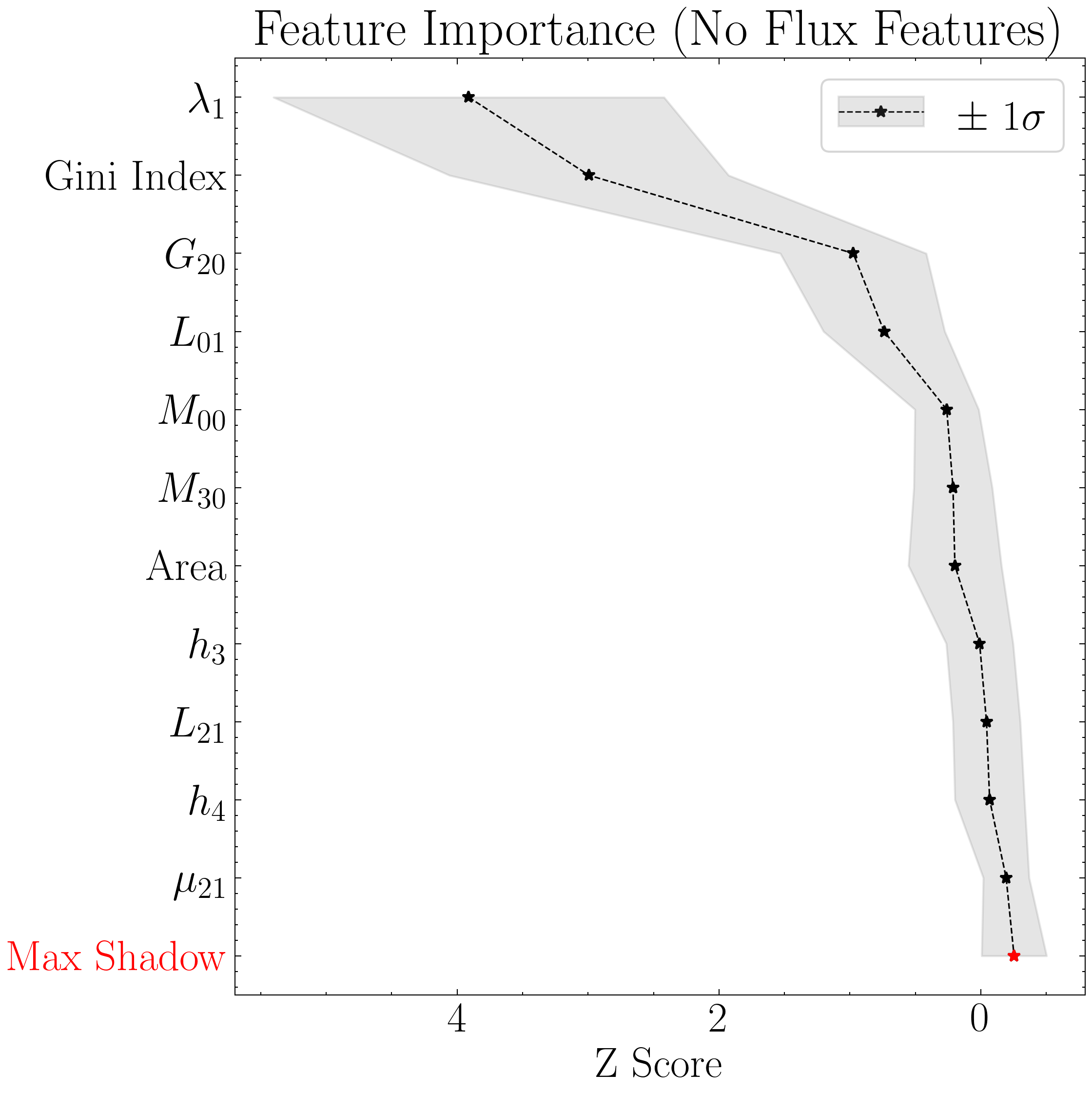
This optimized morphological-only XGBoost model can be downloaded here.
Next we classify the full NDWFS catalog (saved above, see subsection Boötes Morphological Catalog) and compare the results with the adopted XGBoost-8 model.
# Now classify the full NDWFS Bootes catalog

# Load the catalog containing all 2 million other objects, extracted using sig=0.32
other_all = pd.read_csv('Other_Catalog_Master_0.32')

# Remove the 859 OTHER objects that are present in the training set, we will assess these individually using LoO
other_all = other_all[~other_all['obj_name'].isin(df_filtered['obj_name'])]

# Log transform the Hu moments
other_all[hu_cols] = other_all[hu_cols].apply(data_processing.signed_log_transform)

# Omit non-detections
mask = np.where((other_all['area'] != -999) & np.isfinite(other_all['mag']) & np.all(np.isfinite(other_all[[f'Hu{i}' for i in range(1, 8)]]), axis=1))[0]

other_all = other_all.iloc[mask]

# Create the data_x array
other_data_x = np.array(other_all[columns])

# Predict all samples to create a candidates catalog
predictions = model.predict(other_data_x)

# Filter for the positive predictions only (label == 1)
LAB_predictions = np.where(predictions[:,0] == 1)[0]

# Select those probability predictions only and corresponding Bw magnitudes
LAB_predictions_probas = predictions[:,1][LAB_predictions]
mag_candidates = other_all.mag.iloc[LAB_predictions]

# Now load the candidates output by the XGBoost-8 model and saved above (Predictions & LOO CV subsection)
xgboost_8_candidates = pd.read_csv('candidate_catalog_optimized_xgboost_8.csv')
mag_candidates_xgboost8 = xgboost_8_candidates.mag
With the probability scores and corresponding Bw magnitudes, the magnitude distributions and the bin-averaged probability predictions as a function of magnitude.
import matplotlib.pyplot as plt
import scienceplots
plt.style.use("science")
plt.rcParams.update({"font.size": 21})

def step_fraction_hist(ax, x, bins, label, **step_kwargs):
    """
    Helper function to plot the histograms showing the fractional distributions.
    """
    hist, _ = np.histogram(x, bins=bins)
    frac = hist / hist.sum() if hist.sum() > 0 else np.zeros(len(bins) - 1)
    centers = 0.5 * (bins[:-1] + bins[1:])
    ax.step(centers, frac, where="mid", label=f"{label} (n={len(x):,})", **step_kwargs)
    return frac

# Combine the magnitudes from both candidate sets to compute global min/max for bins
all_ = np.concatenate([mag_candidates, mag_candidates_xgboost8])
min_, max_ = np.nanmin(all_), np.nanmax(all_)

# Set bins
num_bins = 100
bins = np.linspace(min_, max_, num_bins + 1)

# Plot
fig, ax = plt.subplots(figsize=(8, 8))
step_fraction_hist(ax, mag_candidates, bins, r"Model Without Flux Features", lw=2.5, ls="-")
step_fraction_hist(ax, mag_candidates_xgboost8, bins, f'XGBoost-8', lw=2.5, ls="-.")
ax.set_xlabel(r'$B_W$ Mag'); ax.set_ylabel('Fraction of Objects')
ax.set_xlim(bins[0], bins[-1])
ax.set_title('LAB Initial Candidates')
ax.legend(handlelength=1.2, frameon=True, fancybox=True)
ax.set_ylim((0,0.21))
plt.tight_layout()
plt.show()
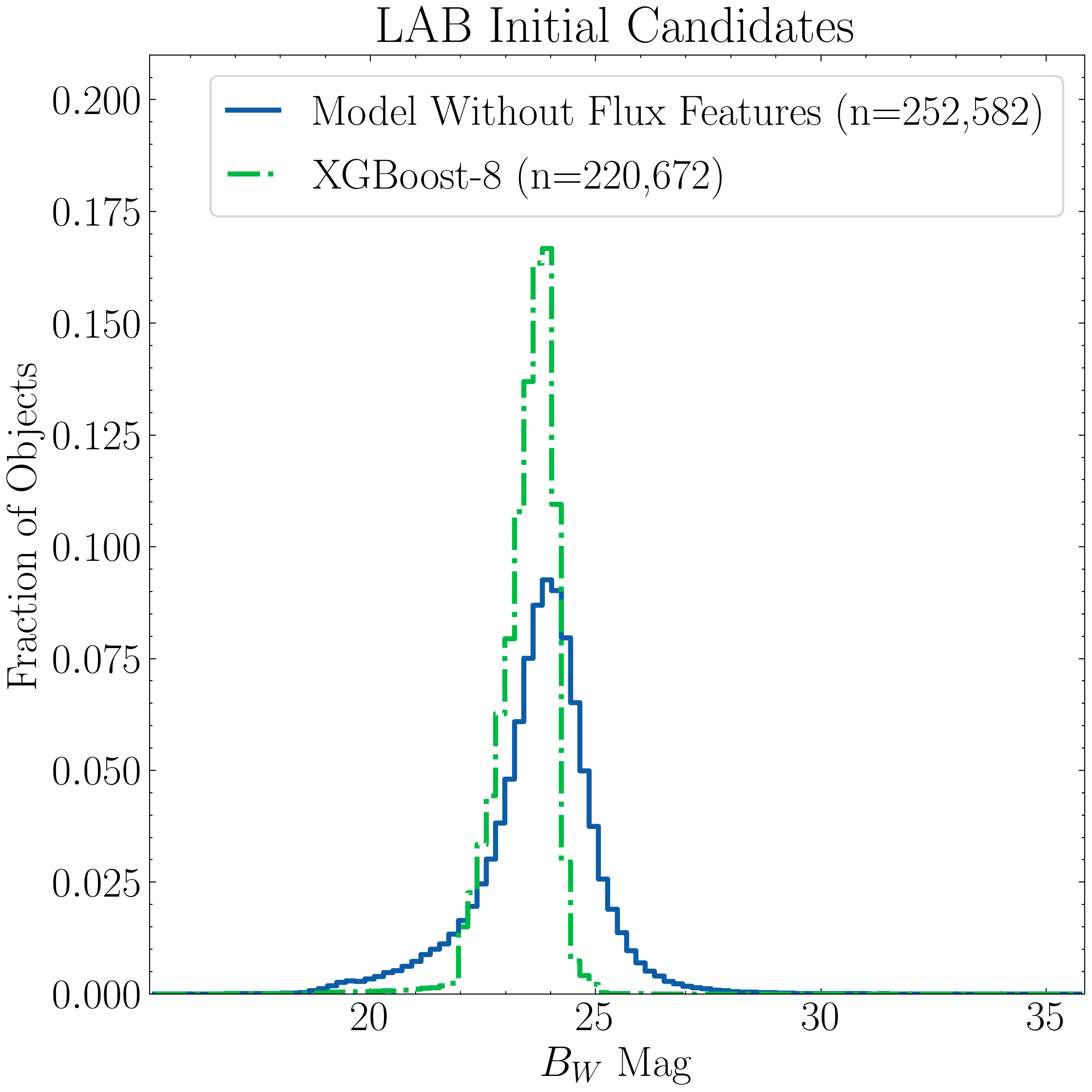
Finally we analyze the correlation between the Bw magnitude of a source and its probability prediction score.
# Load the XGBoost-8 model and re-do the predictions on the full dataset
xgboost_8_model = ensemble_model.Classifier()
xgboost_8_model.load('ensemble_model_xgb_boruta_xgb')

# Need all features in this case
columns = [
    'mag', 'mag_err',
    'M00', 'M10', 'M01', 'M20', 'M11', 'M02', 'M30', 'M21', 'M12', 'M03',
    'mu20', 'mu11', 'mu02', 'mu30', 'mu21', 'mu12', 'mu03',
    'G10', 'G01', 'G20', 'G11', 'G02', 'G30', 'G21', 'G12', 'G03',
    'Hu1', 'Hu2', 'Hu3', 'Hu4', 'Hu5', 'Hu6', 'Hu7',
    'L00', 'L10', 'L01', 'L20', 'L11', 'L02', 'L30', 'L21', 'L12', 'L03',
    'area', 'covar_sigx2', 'covar_sigy2', 'covar_sigxy', 'covariance_eigval1', 'covariance_eigval2',
    'cxx', 'cxy', 'cyy', 'eccentricity', 'ellipticity', 'elongation',
    'equivalent_radius', 'fwhm', 'gini', 'orientation', 'perimeter',
    'semimajor_sigma', 'semiminor_sigma', 'max_value', 'min_value'
]

other_data_x = np.array(other_all[columns])

# Predict all samples to create a candidates catalog
predictions_xgboost8 = xgboost_8_model.predict(other_data_x)

# If the predicted label is 0 (negative), the positive class prob is (1 - prob).
p1 = np.where(predictions[:, 0] == 1, predictions[:, 1], 1 - predictions[:, 1])
p2 = np.where(predictions_xgboost8[:, 0] == 1, predictions_xgboost8[:, 1], 1 - predictions_xgboost8[:, 1])

# Magnitudes for the entire catalog
mag_val = other_all["mag"].to_numpy(dtype=float)

# Set global range for the bins
valid_p = np.concatenate([p1[np.isfinite(p1)], p2[np.isfinite(p2)]])
min_prob = np.min(valid_p)
max_prob = np.max(valid_p)

# Using 49 bins (50 edges)
bins = np.linspace(min_prob, max_prob, 50)
bin_centers = (bins[:-1] + bins[1:]) / 2

def get_binned_stats(probs, values, bins):
    """
    Helper function to define the bin averages and variance
    """

    avg_arr, std_arr = [], []

    # Compute the mean and std for each bin
    for i in range(len(bins) - 1):
        # Create the mask for specific bin slice
        mask_bin = (probs >= bins[i]) & (probs < bins[i+1])
        valid_indices = mask_bin & np.isfinite(values)
        subset = values[valid_indices]

        avg_arr.append(np.mean(subset))
        std_arr.append(np.std(subset))

    return np.array(avg_arr), np.array(std_arr)

# Calculate the bin stats
mean1, std1 = get_binned_stats(p1, mag_val, bins)
mean2, std2 = get_binned_stats(p2, mag_val, bins)

# Plot
fig, ax = plt.subplots(figsize=(8, 8))

# Model 1, No Flux Features
mask1 = np.isfinite(mean1)
ax.plot(bin_centers[mask1], mean1[mask1], lw=1.6, color='C0', label=f"Model Without Flux Features")
ax.fill_between(
    bin_centers[mask1],
    mean1[mask1] - std1[mask1],
    mean1[mask1] + std1[mask1],
    color='C0', alpha=0.3
)

# Model 2, XGBoost-8
mask2 = np.isfinite(mean2)
ax.plot(bin_centers[mask2], mean2[mask2], lw=1.6, ls="-.", color='C1', label=f"XGBoost-8")
ax.fill_between(
    bin_centers[mask2],
    mean2[mask2] - std2[mask2],
    mean2[mask2] + std2[mask2],
    color='C1', alpha=0.3
)

# Labels and formatting
ax.set_xlabel(r"$P(y =$ LAB $\mid \mathbf{X})$")
ax.set_ylabel(r"$B_W$ Mag")
ax.set_xlim(0.0, 1.0)
ax.invert_yaxis()
ax.set_title(r"Impact of Flux Features on Classification")
ax.legend(handlelength=1.2, frameon=True, fancybox=True, loc='lower right')
plt.tight_layout()
plt.show()
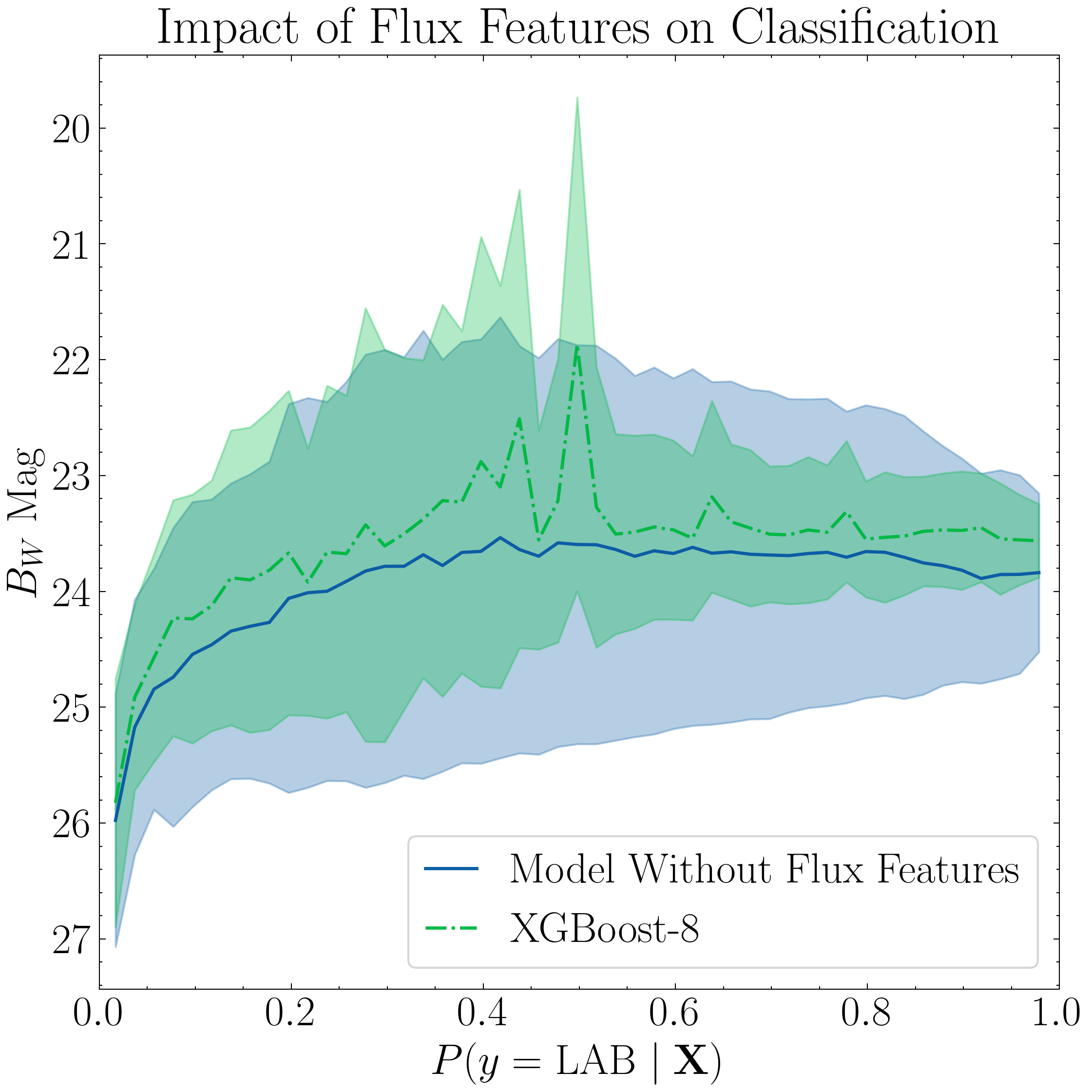
Additional Robustness Experiment
Given our limited training data, to take advantage of the full training signal, we adopt an internal 10-fold cross-validation strategy to assess the performance of the six models presented in Figure 2. However, to guard against overfitting we conduct a held-out test experiment, repeating our optimal detection threshold analysis but with a 70/30 train/test split.
import numpy as np
import pandas as pd
from pyBIA import data_processing, ensemble_model

from sklearn.model_selection import train_test_split, StratifiedKFold, cross_validate
from sklearn.metrics import accuracy_score, f1_score
from sklearn.preprocessing import StandardScaler
from sklearn.pipeline import Pipeline
from sklearn.base import clone

# Same set up as before
SEED_NO = 1909
sigs = np.around(np.arange(0.1, 1.51, 0.01), decimals=2)
nsig_path = 'nsigs/'

columns = [
    'mag', 'mag_err',
    'M00', 'M10', 'M01', 'M20', 'M11', 'M02', 'M30', 'M21', 'M12', 'M03',
    'mu20', 'mu11', 'mu02', 'mu30', 'mu21', 'mu12', 'mu03',
    'G10', 'G01', 'G20', 'G11', 'G02', 'G30', 'G21', 'G12', 'G03',
    'Hu1', 'Hu2', 'Hu3', 'Hu4', 'Hu5', 'Hu6', 'Hu7',
    'L00', 'L10', 'L01', 'L20', 'L11', 'L02', 'L30', 'L21', 'L12', 'L03',
    'area', 'covar_sigx2', 'covar_sigy2', 'covar_sigxy', 'covariance_eigval1', 'covariance_eigval2',
    'cxx', 'cxy', 'cyy', 'eccentricity', 'ellipticity', 'elongation',
    'equivalent_radius', 'fwhm', 'gini', 'orientation', 'perimeter',
    'semimajor_sigma', 'semiminor_sigma', 'max_value', 'min_value'
]

# The six models (from Fig. 2)
classifiers = ['tree', 'rf', 'xgb', 'logreg', 'svc', 'nn']
all_metrics = {
    clf: {
        "nsig": [],
        "cv_accuracy": [], "cv_accuracy_std": [],
        "cv_f1": [], "cv_f1_std": [],
        "test_accuracy": [], "test_accuracy_std": [],
        "test_f1": [], "test_f1_std": []
    }
    for clf in classifiers
}

# No imputation since all features are valid
impute = False

# Number of cross-validation folds for internal train assesment
num_cv_folds = 10

# Number of random 70/30 train/test split partitions
N_REPEATS = 10

for sig in sigs:

    # Load the particular file
    df = pd.read_csv(nsig_path + '_Bw_training_set_nsig_' + str(sig))

    # Log transform the Hu features
    hu_cols = ['Hu1', 'Hu2', 'Hu3', 'Hu4', 'Hu5', 'Hu6', 'Hu7']
    df[hu_cols] = df[hu_cols].apply(data_processing.signed_log_transform)

    # Mask away the non-detections
    mask = np.where(
        (df['area'] != -999) &
        np.isfinite(df['mag']) &
        np.all(np.isfinite(df[[f'Hu{i}' for i in range(1, 8)]]), axis=1)
    )[0]

    # Training set
    blob_index  = np.where(df['flag'].iloc[mask] == 1)[0]
    other_index = np.where(df['flag'].iloc[mask] == 0)[0]
    df_filtered = df.iloc[mask[np.concatenate((blob_index, other_index[:len(blob_index)]))]]

    # Shuffle once per sigma_det to avoid any ordering artifacts
    df_filtered = df_filtered.sample(frac=1, random_state=SEED_NO).reset_index(drop=True)
    X_full = df_filtered[columns].to_numpy()
    y_full = df_filtered["flag"].to_numpy().astype(int)

    # Loop through and assess each engine
    for clf_name in classifiers:
        rep_cv_acc, rep_cv_f1 = [], []
        rep_test_acc, rep_test_f1 = [], []
        for rep in range(N_REPEATS):
            split_seed = SEED_NO + rep # To ensure each train/test split is unique
            X_train, X_test, y_train, y_test = train_test_split(
                X_full, y_full,
                test_size=0.30,
                random_state=split_seed,
                shuffle=True,
                stratify=y_full
            )

            # For test evaluation, need to scale using the scaler fitted on train data (only for logred, svc, and nn)
            if clf_name in ["logreg", "svc", "nn"]:
                scaler = StandardScaler().fit(X_train)
                X_train_fit = scaler.transform(X_train)
                X_test_fit  = scaler.transform(X_test)
            else:
                X_train_fit, X_test_fit = X_train, X_test

            # Instantiate the Classifier and train
            wrapper = ensemble_model.Classifier(X_train_fit, y_train, impute=impute)
            wrapper.clf = clf_name
            wrapper.create(overwrite_training=False)

            # Hold out test set metrics
            y_pred = wrapper.model.predict(X_test_fit)
            rep_test_acc.append(accuracy_score(y_test, y_pred))
            rep_test_f1.append(f1_score(y_test, y_pred, zero_division=0))

            # Internal metrics based on 10-fold CV
            class_counts = np.bincount(y_train, minlength=2)
            min_class = int(class_counts.min())
            n_splits = min(num_cv_folds, min_class)
            if n_splits < 2:
                continue

            cv_splitter = StratifiedKFold(n_splits=n_splits, shuffle=True, random_state=split_seed)
            # CV for scaled models
            est = clone(wrapper.model)
            if clf_name in ["logreg", "svc", "nn"]:
                est_cv = Pipeline([("scaler", StandardScaler()), ("clf", est)])
                cv_X = X_train
            else:
                est_cv = est
                cv_X = X_train

            # Cross-validation
            cv = cross_validate(
                est_cv,
                cv_X, y_train,
                cv=cv_splitter,
                scoring=["accuracy", "f1"],
                n_jobs=-1
            )

            # Save train and test metrics for this particular split
            rep_cv_acc.append(cv["test_accuracy"].mean())
            rep_cv_f1.append(cv["test_f1"].mean())

        # Save all metrics for this classifier
        all_metrics[clf_name]["nsig"].append(sig)
        all_metrics[clf_name]["cv_accuracy"].append(np.mean(rep_cv_acc) if rep_cv_acc else np.nan)
        all_metrics[clf_name]["cv_accuracy_std"].append(np.std(rep_cv_acc) if rep_cv_acc else np.nan)
        all_metrics[clf_name]["cv_f1"].append(np.mean(rep_cv_f1) if rep_cv_f1 else np.nan)
        all_metrics[clf_name]["cv_f1_std"].append(np.std(rep_cv_f1) if rep_cv_f1 else np.nan)
        all_metrics[clf_name]["test_accuracy"].append(np.mean(rep_test_acc) if rep_test_acc else np.nan)
        all_metrics[clf_name]["test_accuracy_std"].append(np.std(rep_test_acc) if rep_test_acc else np.nan)
        all_metrics[clf_name]["test_f1"].append(np.mean(rep_test_f1) if rep_test_f1 else np.nan)
        all_metrics[clf_name]["test_f1_std"].append(np.std(rep_test_f1) if rep_test_f1 else np.nan)

# Flatten the dict and save to a dataframe
rows = []
for clf_name, metrics in all_metrics.items():
    # 'nsig' dictates the number of data points per classifier
    for i in range(len(metrics['nsig'])):
        row = {'classifier': clf_name}
        for metric_name, values_list in metrics.items():
            row[metric_name] = values_list[i]
        rows.append(row)

df_results = pd.DataFrame(rows)
df_results.to_csv('cv_vs_test_metrics.csv', index=False)
The dataframe saved above can be downloaded here.
Below we plot the results of this robustness experiment.
import pandas as pd
import matplotlib.pyplot as plt
import scienceplots
plt.style.use('science')
plt.rcParams.update({'font.size':21,})

# Load the saved dataframe
df_results = pd.read_csv('cv_vs_test_metrics.csv')


# Plot one subplot per model to show both train and test scores
fig, axes = plt.subplots(2, 3, figsize=(16, 10), sharex=True, sharey=True)
axes = axes.flatten()

# So the classifier names are consistent with Fig. 2
title_map = {
    'logreg': 'LogReg',
    'nn': 'MLP',
    'rf': 'RF',
    'svc': 'SVC',
    'tree': 'Tree',
    'xgb': 'XGBoost'
}

# Loop through each classifier and plot train and test scores
for idx, clf in enumerate(df_results['classifier'].unique()):
    ax = axes[idx]
    df_clf = df_results[df_results['classifier'] == clf].reset_index(drop=True)
    ax.plot(df_clf['nsig'], df_clf['cv_f1'], label='Train (10-Fold CV)', color='blue', linewidth=1.5)
    ax.fill_between(df_clf['nsig'], df_clf['cv_f1'] - df_clf['cv_f1_std'], df_clf['cv_f1'] + df_clf['cv_f1_std'], color='blue', alpha=0.2)
    ax.plot(df_clf['nsig'], df_clf['test_f1'], label='Hold-out Test', linestyle='--', color='red', linewidth=1.5)
    ax.set_title(title_map.get(clf, clf))
    if idx == 1: ax.legend(loc='lower center', handlelength=1, frameon=True, fancybox=True)
    if idx == 0 or idx == 3: ax.set_ylabel('F1 Score')
    if idx >= 3: ax.set_xlabel(r'$\sigma_{\rm det}$')

plt.tight_layout()
plt.show()
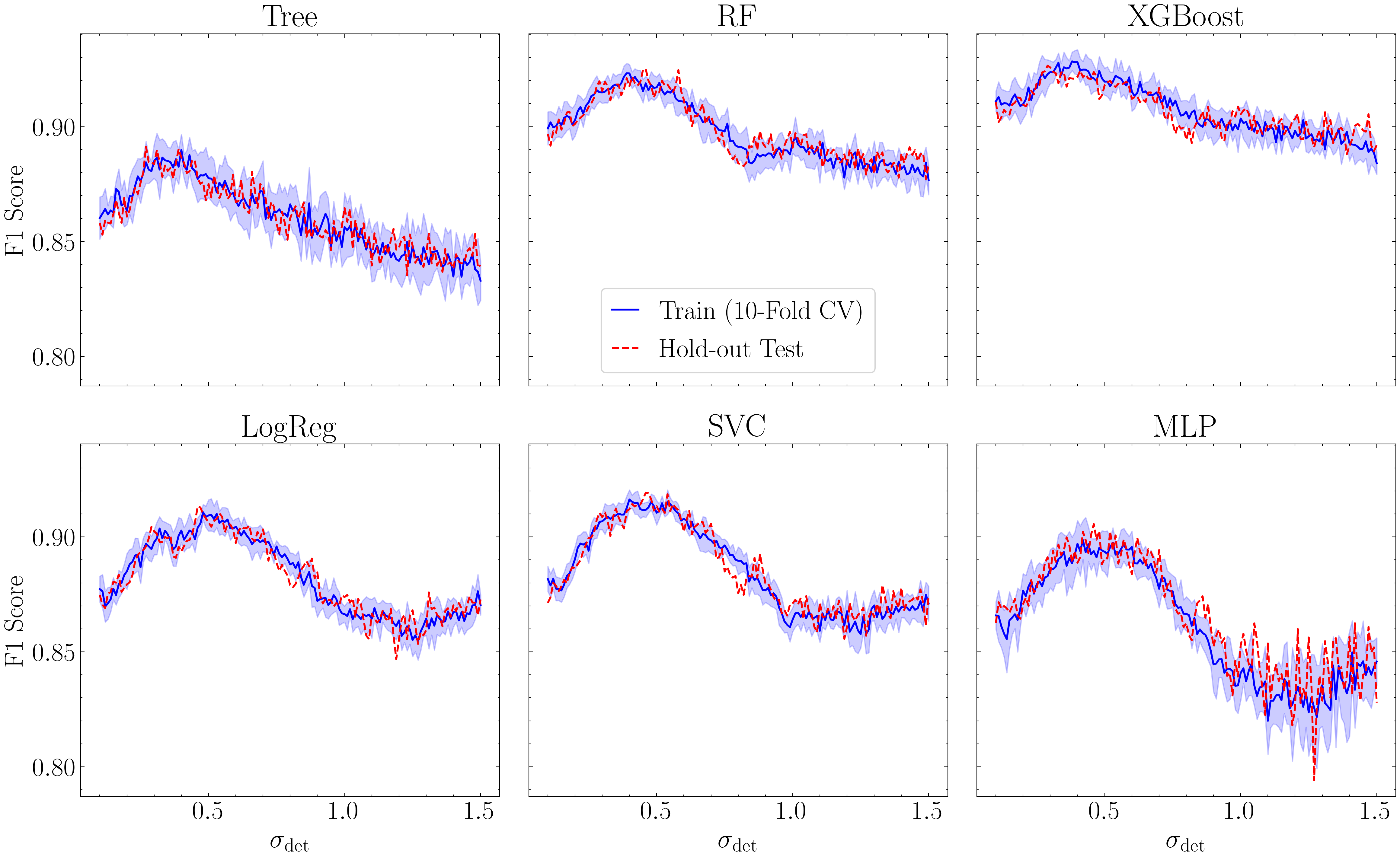
These results are consistent with Fig 2, demonstrating that our internal cross-validation did not introduce severe overfitting. Using the same segmentation detection threshold of 0.32, we now tune the model using the same optimization routine (BorutaSHAP with XGBoost estimator + Optuna), but also using a 70/30 train/test partition.
import numpy as np
import pandas as pd
from pyBIA import data_processing, ensemble_model
from sklearn.model_selection import train_test_split
from sklearn.metrics import accuracy_score, f1_score

# Same set up as before
SEED_NO = 1909
sigs = np.around(np.arange(0.1, 1.51, 0.01), decimals=2)
nsig_path = 'nsigs/'

columns = [
    'mag', 'mag_err',
    'M00', 'M10', 'M01', 'M20', 'M11', 'M02', 'M30', 'M21', 'M12', 'M03',
    'mu20', 'mu11', 'mu02', 'mu30', 'mu21', 'mu12', 'mu03',
    'G10', 'G01', 'G20', 'G11', 'G02', 'G30', 'G21', 'G12', 'G03',
    'Hu1', 'Hu2', 'Hu3', 'Hu4', 'Hu5', 'Hu6', 'Hu7',
    'L00', 'L10', 'L01', 'L20', 'L11', 'L02', 'L30', 'L21', 'L12', 'L03',
    'area', 'covar_sigx2', 'covar_sigy2', 'covar_sigxy', 'covariance_eigval1', 'covariance_eigval2',
    'cxx', 'cxy', 'cyy', 'eccentricity', 'ellipticity', 'elongation',
    'equivalent_radius', 'fwhm', 'gini', 'orientation', 'perimeter',
    'semimajor_sigma', 'semiminor_sigma', 'max_value', 'min_value'
]

# Load training data, using the optimal detection threshold chosen based on Fig. 2
sig = 0.32
df = pd.read_csv(nsig_path + '_Bw_training_set_nsig_' + str(sig))

# Log transform the Hu features
hu_cols = ['Hu1', 'Hu2', 'Hu3', 'Hu4', 'Hu5', 'Hu6', 'Hu7']
df[hu_cols] = df[hu_cols].apply(data_processing.signed_log_transform)

# Mask detections
mask = np.where(
    (df['area'] != -999) &
    np.isfinite(df['mag']) &
    np.all(np.isfinite(df[[f'Hu{i}' for i in range(1, 8)]]), axis=1)
)[0]

# Training set for this sigma threshold
blob_index  = np.where(df['flag'].iloc[mask] == 1)[0]
other_index = np.where(df['flag'].iloc[mask] == 0)[0]
df_filtered = df.iloc[mask[np.concatenate((blob_index, other_index[:len(blob_index)]))]]

# Shuffle
df_filtered = df_filtered.sample(frac=1, random_state=SEED_NO).reset_index(drop=True)
X_full = df_filtered[columns].to_numpy()
y_full = df_filtered["flag"].to_numpy().astype(int)

# Train/test split
split_seed = 1909
X_train, X_test, y_train, y_test = train_test_split(
    X_full, y_full,
    test_size=0.30,
    random_state=split_seed,
    shuffle=True,
    stratify=y_full
)

# Train and tune an XGBoost model, same set up as before
SEED_NO = 1909 # The seed number that will initialize the stochastic process (e.g., model training)
clf = 'xgb' # The classification model that will be trined, options are: 'xgb', 'rf' and 'nn'
impute = False # Whether to impute missing values (NaN)
optimize = True # Will enable the optimization routine
scoring_metric = 'f1' # The optimization trials will be assessed according to the F1 Score
opt_cv = 10 # The number of folds to perform during cross validation, ONLY used during optimization (`optimize`=True)
boruta_trials = 100 # Number of feature selection trials to perform (This is fast especially with `boruta_model`='xgb')
boruta_model = 'xgb' # The model to use when assessing feautre importances during feature selection (either 'rf' or 'xgb', DOES NOT have to match the `clf`)
n_iter = 100 # Number of hyperparameter optimization trials to perform, can set to 0 to disable hyperparam tuning
limit_search = True # Set to False to expand the hyperparameter search space (will take longer)

# Instantiate the Classifier
model = ensemble_model.Classifier(
    X_train,
    y_train,
    clf=clf,
    impute=impute,
    optimize=optimize,
    boruta_trials=boruta_trials,
    boruta_model=boruta_model,
    n_iter=n_iter,
    scoring_metric=scoring_metric,
    opt_cv=opt_cv,
    limit_search=limit_search,
    SEED_NO=SEED_NO
    )

model.save('model_train_test_split')

# Plot roc curve
model.plot_roc_curve()

# Plot feature importance
columns_formatted = [
    #r'$B_W$ Mag', r'$B_W$ MagErr',
    r'$M_{00}$', r'$M_{10}$', r'$M_{01}$', r'$M_{20}$', r'$M_{11}$', r'$M_{02}$', r'$M_{30}$', r'$M_{21}$', r'$M_{12}$', r'$M_{03}$',
    r'$\mu_{20}$', r'$\mu_{11}$', r'$\mu_{02}$', r'$\mu_{30}$', r'$\mu_{21}$', r'$\mu_{12}$', r'$\mu_{03}$',
    r'$G_{10}$', r'$G_{01}$', r'$G_{20}$', r'$G_{11}$', r'$G_{02}$', r'$G_{30}$', r'$G_{21}$', r'$G_{12}$', r'$G_{03}$',
    r'$h_1$', r'$h_2$', r'$h_3$', r'$h_4$', r'$h_5$', r'$h_6$', r'$h_7$',
    r'$L_{00}$', r'$L_{10}$', r'$L_{01}$', r'$L_{20}$', r'$L_{11}$', r'$L_{02}$', r'$L_{30}$', r'$L_{21}$', r'$L_{12}$', r'$L_{03}$',
    'Area', r'$\sigma^2(x)$', r'$\sigma^2(y)$', r'$\sigma^2(xy)$', r'$\lambda_1$', r'$\lambda_2$', r'$C_{xx}$', r'$C_{xy}$', r'$C_{yy}$',
    'Eccentricity', 'Ellipticity', 'Elongation', 'Equiv. Radius', 'FWHM', 'Gini Index', 'Orientation', 'Perimeter',
    r'$\sigma_{\rm major}$', r'$\sigma_{\rm minor}$'#, 'Max Value', 'Min Value'
]

model.plot_feature_opt(feat_names=columns_formatted)

# Now evaluate the held-out test set
y_pred = model.model.predict(X_test[:,model.feats_to_use])
print('Hold-out test F1 score', f1_score(y_test, y_pred, zero_division=0))
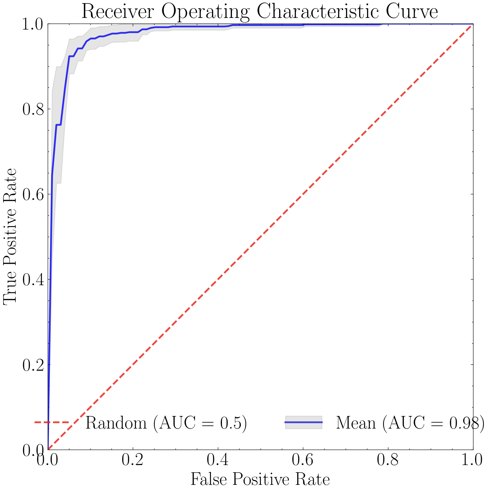
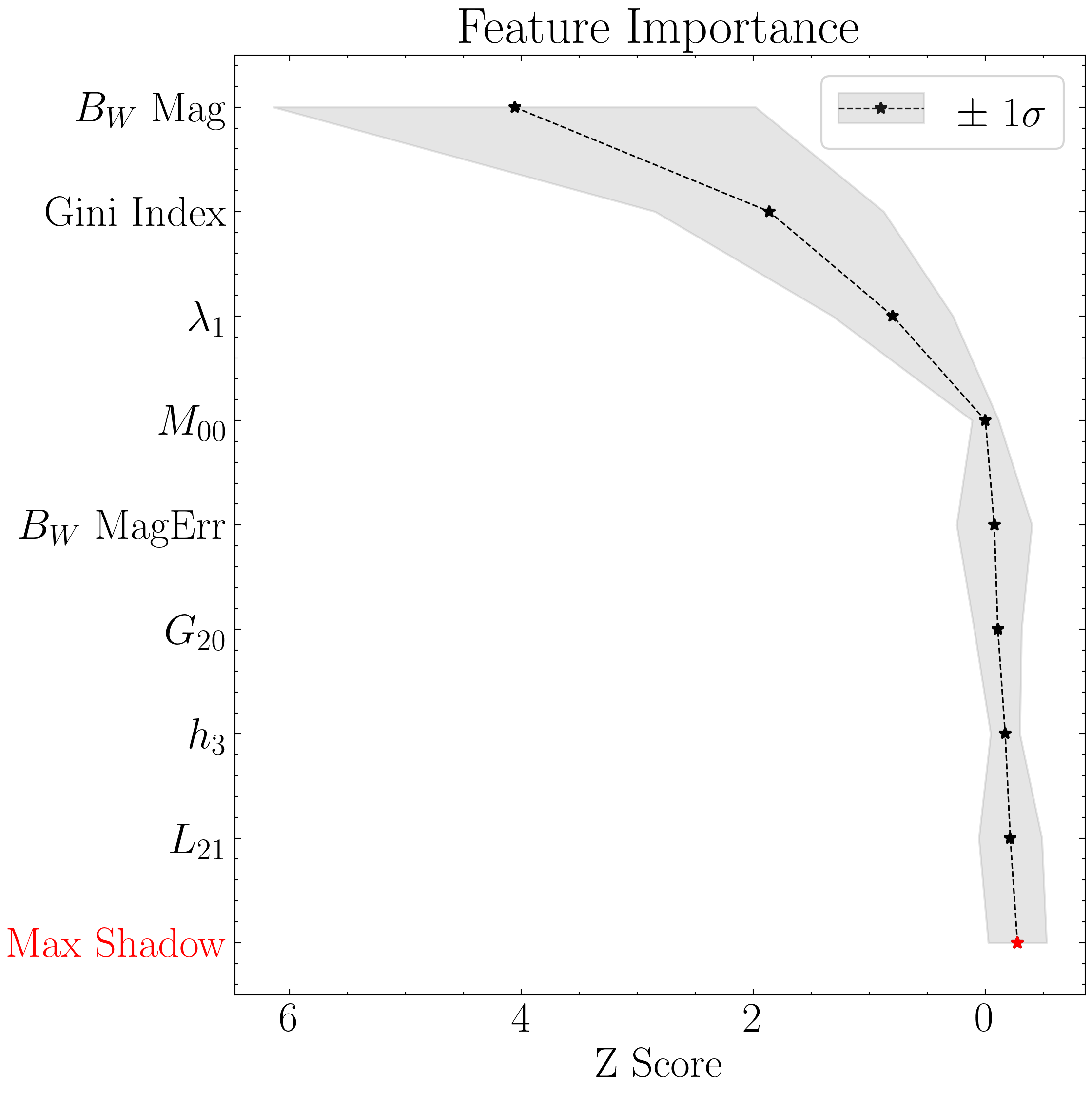
This tuned model, trained on 70% of the data, yields an F1 score of 0.9162 on the hold-out test set an 10-fold cross-validated F1 score of 0.939 on the training set (compared to 0.9336 for the original XGBoost-8 model that was trained using the full dataset).
The cross-validated ROC curve yields an AUC of 0.98, consistent with the original XGBoost-8 model. Furthermore, in this experiment, the selected features are very similar to XGBoost-8. The top three features remain the same, and 6 of the 8 features from the original XGBoost-8 model are retained in this new training configuration.
This model can be downloaded here.